
Overview
At the core of nearly all procedural terrain generation is noise. Not to be confused with audio/signal noise, noise refers to the randomness, or more specifically pseudorandomness, that allows for the generation of new content. Whereas most functions adhere to generating predictable patterns expected by users, randomness purposefully attempts to subvert expectations by creating unpredictable outcomes. While achieving unpredictability may simply involve increasing layers of arbitrary complexity, natural terrain isn’t defined by absolute randomness. Rather, a level of predictability is commonplace; one would expect rough rocky terrain along mountain ridges and smooth sandy deserts. To capture such patterns without predefining terrain requires a balance between randomness and predictability.
Background
Unlike my other articles, I present no new strategy in basic noise generation. With the popularization of noise generation techniques through the quintissential paradigm of terrain generation, Minecraft, noise generation for the purpose of procedural terrains is a well-documented idea. Various strategies have been proposed and implemented applying various forms of procedural noise all to varying degrees of proficiency.
Instead, through a series of reflections and justifications, I plan to discuss the specific approach to noise sampling implemented as to lay a foundation for further articles discussing noise-based terrain generation. In the process I also hope to provide an evaluation of certain strategies used in transforming noise into terrain.
Specifications
With regards to terrain generation, it is important to consider noise-generation in the format that it will be commonly viewed in. For images, height-maps, and textures, this often requires a 2D representation of noise, which requires a minimum of two axis parameters to deliniate the location of the sample. Evaluating the efficiency of a noise-algorithm will appear more reasonable when discussing a measurement notable in the fashion the noise is meant to be displayed. Discussion of 2D noise representation is more sensible when relating the change in noise to its 2D position.
Previously I discussed the need for terrain-generation to be deterministic and this applies especially to noise sampling. For clarification, all computing systems are deterministic, built upon functions that provide consistent outputs to identical inputs; the only truely non-deterministic aspect is the user’s inputs. What being determinstic here actually refers to is that all factors affecting an output(all its parameters) are exposed on a top-level. This way, one can be certain of a predictable response as all aspects capable of producing different behavior is accessible to them–a given seed(collection of these factors) will always elicit the same output.
Solution
Simplex Noise
The base of all complex noise generation is a noise-generation algorithm. In the simplest of terms, noise generation is a function that recieves an argument and returns an output. The function does not store information regarding every possible argument, but transforms all the arguments based on a set amount of instructions. For noise, this transformation attempts to subvert human expectation as to present itself as random.
To start, a random number generator often refers to a simple 1D noise-algorithm that produces a seemingly random output from a seed, which will be a number that represents the position along a 1D axis. For floating-point, a common approach is a series of arithmetic, trig and modulo operations, such as frac(sin(seed) * 43758.5453123) and then the result may be scaled by the desired range, and integer representation often involves a series of prime-xors and bit-shifts to randomize the bitmap: (seed ^ (seed >> 16) * 0x85ebca6b) where the result can be scaled down by the range of the specific representation. For a finite 2D grid, the major axis may be multiplied by the capacity of the minor axis to create a unique seed for every sample location, but more commonly an(in effect) infinite 2D map may be created by randomizing the major and minor coordinates and then randomizing the sum of their output: rand(rand(x) + rand(y))
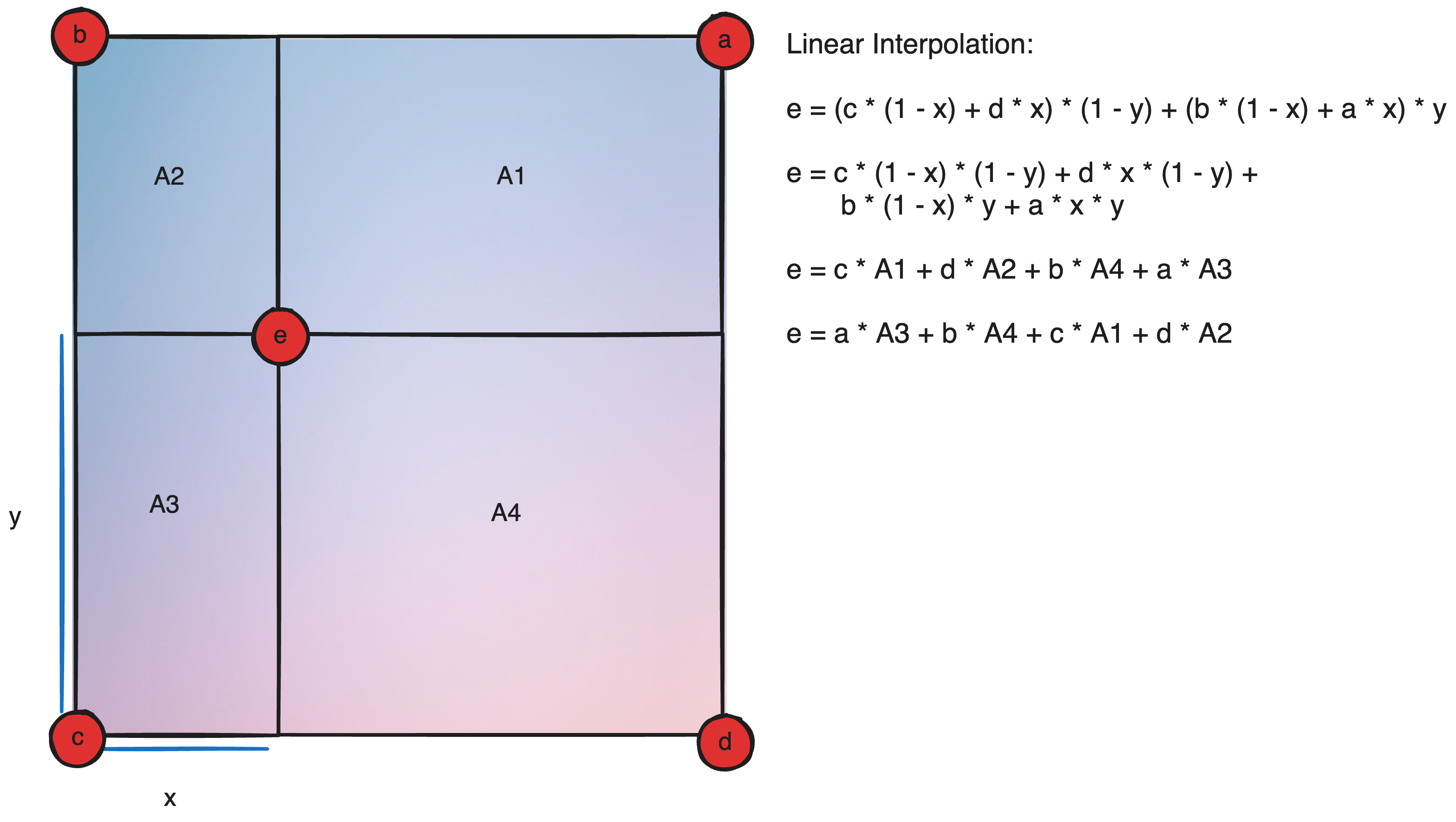
Yay we’ve made some… grainy noise? While this is a start, it’s not very useful for large terrains as it’s far too random and coarse. A way to compensate is to scale up the noise, and then reinterpret every coordinate via a binlinear interpolation of the nearest 4 samples; we can enlarge and blur the noisemap.
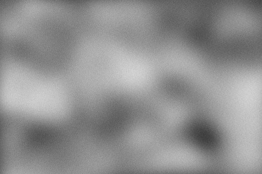
Porting this directly, there is a glaring problem. Though the ground is connected, it is mostly flat and uninteresting. But more importantly, the terrain is not smooth along the edges of our enlarged sample or at the sample positions.
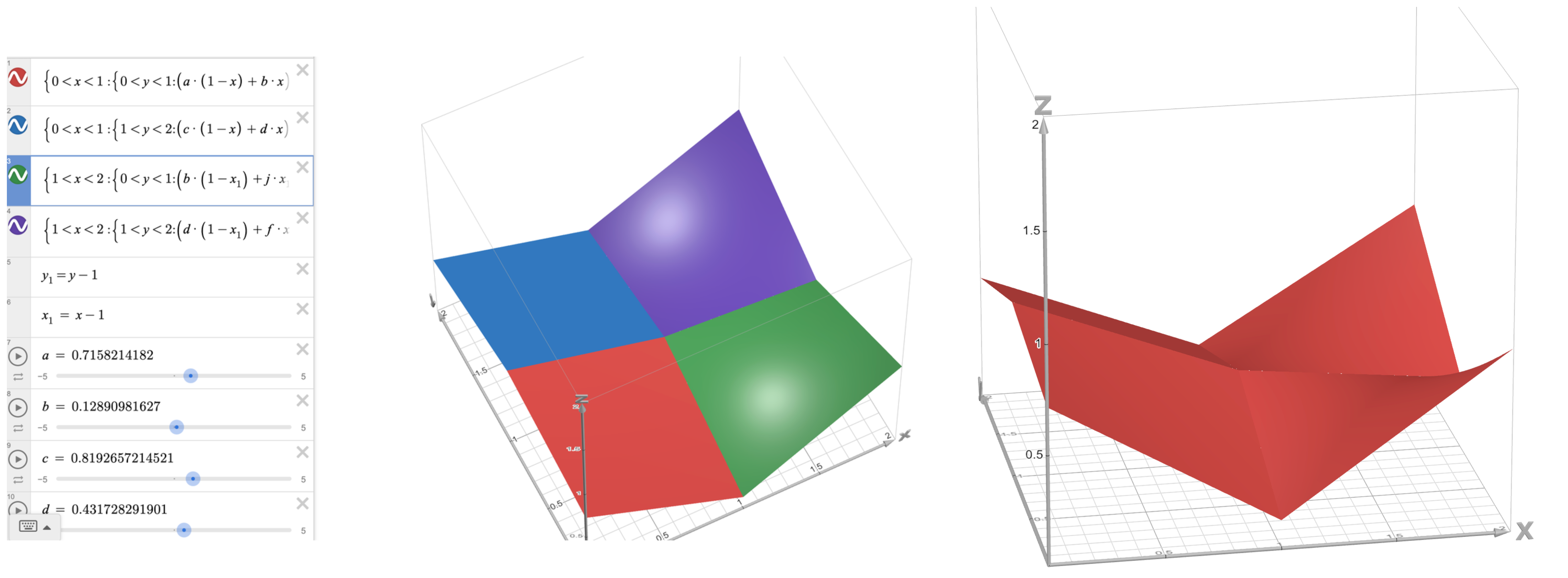
The first problem comes from the nature of how we’re blurring it. Standard blurring, or as I previously referred to as bilinear interpolation, is called blinear particularly because the slope is linear along any straight axis. Another way to say the slope is linear is that the first derivative is constant–it would be much more fun if the function were of a higher order of differentiality such that the ground curved between samples.
The second problem, which we described as not being smooth is better reworded as the derivative being discontinuous, or that the the first derivative changes abruptly across the edge. Ideally to create smooth terrain, not only do we need the first derivative to be continous, but the second derivative must approach zero such that there are no concentrated regions of slope change.
In 1983, Ken Perlin created the famous Perlin Noise algorithm to resolve these problems. He did so by replacing the linear equation used in traditional bilinear interpolation, (a * (1-t) + b * t) | 0 < t < 1 with a fifth order polynomial, f(t) = 6t5 - 15t4 + 10t3, a specific function of a smooth increasing curve from 0->1. In mathematical terms, in the range 0->1, the first derivative is positive & the only zeroes are 0 & 1. This algorithm solved a huge number of problems and concurrently earned international renown resulting in its wide use in procedural terrain generation. However, there were still many areas for improvement.
There are many ways to extend perlin noise for higher dimensions but all of them are problamatic in their own right. For a 3D coordinate, you could sample all combinations of 2D coordinates and then average their sum, or in other words project the coordinate on all axis-orthogonal planes and their reflections and take their sum then divide by 6 (3P2 = 6). However, this has obvious problems where two coordinates align because there will be the same noise generated along both axises as they map to identical projected coordinates. Another option is to modify the Bi-Perlin interpolation to be Tri-Perlin, where 8 points are averaged based off the 3D volume opposite to them. As a rule, interpolation can be extrapolated to any higher dimension with a time complexity of O(2N) where N is the number of dimensions meaning 3D Perlin noise is twice as expensive as traditional 2D noise.
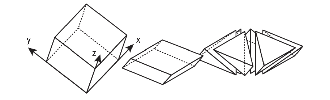
To resolve these issues, Ken Perlin, in 2001, created a Simplex Noise algorithms that boasts to be computationally faster than Perlin noise, scales by O(N2) rather than O(2N), has less directional artifacts, and more hardware intuitive. Instead of interpolating between N-d cubes, simplex-noise evaluates samples on a simplex, or the simplest N-d tilable object. For 1D this is a line with two endpoints, 2D is a triangle with 3 corners, 3D -> tetrahedron with 4 vertices, and though it may be hard to visualize, a 4D simplex is a 4D Hyperhedron with 5 vertices. The trend here is rather than an Nth dimensional cube having 2N vertices, an Nth dimensional simplex has only N+1 vertices. Thus, to determine the noise at a given point, it’s far faster to determine the contributions from a simplex than a cube.

To maintain the deterministic quality of simplex noise, it’s imperative to determine a way to map our samples, which can be defined on an N-d grid aligned graph onto the simplex-tiles. For 1D, a line segment(our simplex) is fully able encapsulate the region between samples. In 2 dimensions, our simplex is a triangle–two of which can be tiled together to create a rhombus which may be skewed to align with grid-aligned samples. In 3D, six tetrahedrons can be arranged to form a rhombohedron. In 4D, 24 4D-simplexes combine to form a grid aligned 4D Hypercube; the number of N-d simplexes in an N-d cube is N!.
However while there are N! possibile simplexes a point in a N-d cube may fall in, determining which simplex a point falls in is rather simple. For a 2D case, consider a grid of integer-aligned squares where each square is divided into two equal isoceles triangles along its positive-slope diagonal. The diagonal of each square has the unique property of defining the line where the fractional x&y components are equivalent meaning all points below it, which is the bottom triangle, have a fractional x-component greater than the fractional y-component and vice versa. By extension,to determine which simplex an n-dimensional point is in reduces to determining the order of increasing fractional axis-components (nPn = n!).
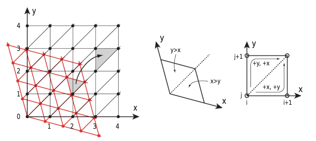
To determine the corner coordinates of the simplex our point is in, we can look again at the diagram.
If we retain the order of increasing fractional axis-components:
i,j,k,… | frac(i) < frac(j) < frac(k) < …
the corners of the simplex can be defined as
floor(i, j, k, …), floor(i + 1, j, k, …), floor(i + 1, j + 1, k, …), floor(i + 1, j + 1, k + 1, …), …
Rather than interpolate between the samples at this point, a final optimization is to weigh each sample by the distance to the simplex-corner from which it originated and taking a summation instead of a direct interpolation. In effect this can achieve the same purpose similar to how one can conduct linear interpolation in an N-d cube by weighing each sample by the N-d volume opposite to it rather than a direct combination of interpolations.
To calculate the (square)distance from each simplex requires a summation of N axis components for N simplex corners resulting in the final time complexity of O(N2). Further information & implementation details on simplex noise can be found here. As of writing this article, Simplex noise represents the state-of-the-art algorithm for 3D noise generation.
Noise Layering
At the moment, the noise we’ve created isn’t very interesting. Between repetitive sloping valleys and hills, there is only a consistent curve; no little bumps or protrusions. This is because simplex, and classical noise, have a defined grid-resolution; random vector samples are only evaluated at grid-aligned positions meaning features can only be as small/big as the grids defining them before they become completely smooth or incoherent grainy noise respectively. Thus, to add variety in detail size–a common approach is to introduce noise octaves.
An octave is, in plain terms, a seperate sample of the underlying base noise-generating algorithm(simplex in this case). Each octave maintains its own arguments that effect how the base noise is sampled, or in other terms, its own conditions that describe the detail level it describes. One octave may scale down the distance between sample-locations, in effect creating large mountains while another may scale up the distance responsible for generating smaller hills.
Though it is possible to expose these octaves and allow them to be individually defined, in practice it is far more commonplace to define a generating function for these octaves. To define a generating function for these octaves, there are, most often, 4 exposed arguments: number of octaves, noise scale, persistance, and lacunarity.
Noise scale and number of octaves are pretty self explanatory. Number of octaves describes how many octaves the generating function should create and, by consequence, directly dictates the workload of noise sampling. The noise scale scales the sampled location supplied to the base noise function(simplex noise) allowing for different sized details. Noise scale and number of octaves remain constant for every octave acting as a constant transformation across all samples.
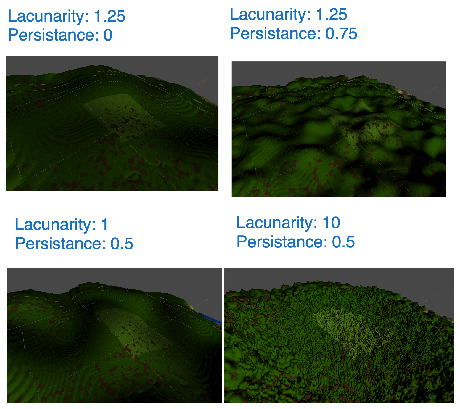
Persistance and Lacunarity, instead, describe how each consecutive noise octave differs from the previous. Because they describe change, in implementation it is commonplace to define other variables representing the actual state, amplitude and frequency respectively, of each octave, where Persistance and Lacunarity describe the percentage change between octaves of amplitude and frequency respectively.
Persistance refers to the change in significance between octaves, or how persistent its features are compared to the previous octave. While this argument can be unrestricted, it is more often than not clamped between zero and one. This is done because it allows us to specify that each preceeding octave is at most as persistant as the current one, allowing the first octave to be defined as maximum amplitude giving finer control over the output range of each octave. Lacunarity refers to the change in base scale. You can think of it as
SampleLocation = Location / Sampling Scale
Sampling Scale = Frequency * Noise Scale
Frequency = Lacunarity ^ (Octave Number)
This is pretty simple to describe as larger frequency means octaves will cover a larger variety of detail levels, and a lower frequency means octaves will sample closer detail levels. Lacunarity is most often clamped to be greater than one, so that the first octave has the smallest sampling scale(biggest features) and features become smaller with each following octave.
Bezier Interpolation Curves
This is better, but the features are very smooth, lumpy, hilly, and don’t possess the sharp ridges, steep drops, and other interesting features that make terrain-generation interesting. Currently, simplex noise aims to provide a smoothed noise-map which directly contradicts with these sharp features which is why they can’t appear. To institute these features we can override reinterpret simplex noise using a custom generation pattern defined through a bezier curve.
Wikipedia defines a Bezier curve as a parametric curve defined by a set of discrete “control points” which contribute to a smooth continuous curve by means of a generation formula. Its goal is to provide a smooth curve which goes through a set of points and whose derivatives(tangents) at those points are assignable. While there is a mathematical derivation for this equation, I find a visual explanation is more helpful here.
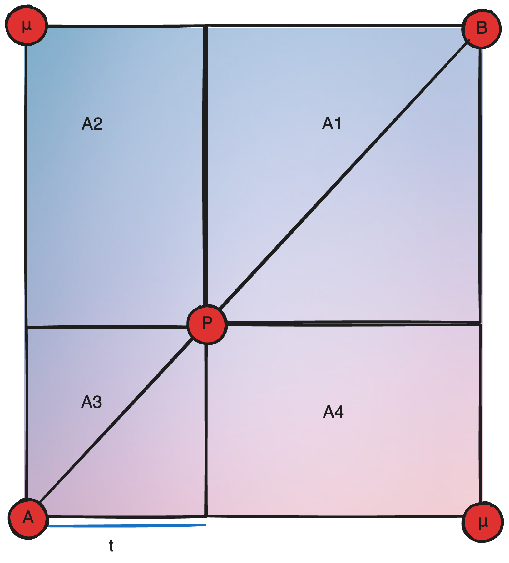
Given 3 2D points A, B and C, and their tangents defined by A0-A1, B0 B1, C0 C1. Our desired curve should look like this.
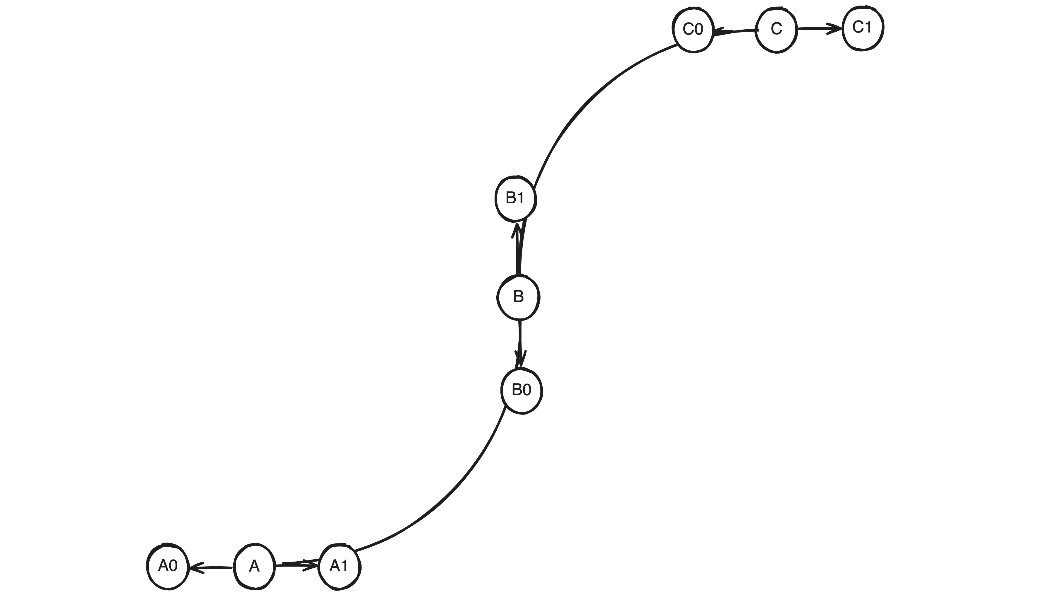
To define a line that passes from A to B, my first thought is to define a parametric function from A to B: A * (1 - t) + B * t, which is a linear interpolation between the two points based on the parameter t which can be thought of as the progress from A to B. While the slopes happen to match up here, we are not following the tangents defined at our control points.
For the tangent to align with the defined control point tangents, we want the derivative to approach the tangent’s derivative as we move closer to the next point. While there is a messy way to do this, a much more elegant solution is to extend each tangent along the distance between the points and average their positions. Then Linearly interpolate between each point and this average, and then linearly interpolate between those values all by the progress. Now that was pretty confusing so I’ll break it down.
Dist = length(B - A)
Anchor = ((A + A1 * Dist) + (B + B0 * Dist)) / 2
Anchor1 = lerp(A, Anchor, t)
Anchor2 = lerp(Anchor, B, t)
output = lerp(Anchor1, Anchor2, t)
lerp(a, b, t) = Linear Interpolate(a, b, t) = a * (1-t) + b * t
Now stacking Linear Interpolations like this isn’t something new. If you remember, I did it earlier to conduct a binary interpolation, which I clarified as weighing each sample by the opposite volume. In this case, since t is the deriving factor in both lerps, one can visualize this as a point moving along a diagonal of a square, where the influence of the avg tangent(μ) is always the square of A2/4, and the position approaches A and B at either end. I don’t know how this is useful, I just thought it was a cool way to think about it.
Visually this works because quadratic lines are curved. You can see how it’s defined it in the diagram below.
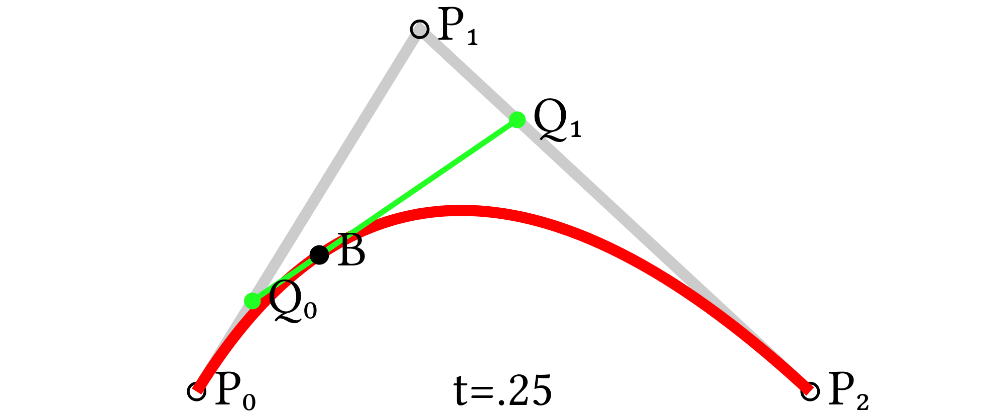
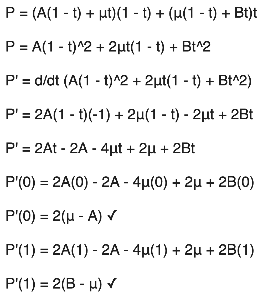
Mathematically, we can prove that we’ve(kind of) achieved our goal of having the slope approach (μ - A) and (B - μ) at either end.
Actually, with the control point definition we’ve defined, a cubic bezier is more fitting where three line segments are defined AA1, A1B0, B0B. This is then reduced to two by interpolating between AA1 to A1B0 and A1B0 to B0B by t and then repeating the same bilinear interpolation. However, this is more computationally intensive while the visual difference is minimal so for the purpose of expedient noise sampling, a quadratic bezier is used.
Conclusion
Thusfar I’ve discussed the layers of complexity that’s applied in the base noise-generation. These strategies are not new innovations I intend to bring forth, but often-used strategies which I simply wished to discuss and document for the purpose of future reference. Going forward, I will rely on this article to discuss more complicated terrain generation, so stay tuned!
Code Source
Optimized HLSL Parallel Implementation
1 | float snoise(float3 v) |