
Overview
At the core of nearly all procedural terrain generation is noise. Not to be confused with audio/signal noise, noise refers to the randomness, or more specifically pseudorandomness, that allows for the generation of new content. Whereas most functions adhere to generating predictable patterns expected by users, randomness purposefully attempts to subvert expectations by creating unpredictable outcomes. While achieving unpredictability may simply involve increasing layers of arbitrary complexity, natural terrain isn’t defined by absolute randomness. Rather, a level of predictability is commonplace; one would expect rough rocky terrain along mountain ridges and smooth sandy deserts. To capture such patterns without predefining terrain requires a balance between randomness and predictability.
Background
Previously, the process of noise sampling, various techniques for optimizing, smoothing, and adding variation, was investigated as a foundation for further discussion of its application. Now that there’s a basis for discussion, Base Generation will focus on the application and use of Noise-Based Terrain Generation, as well as closely-related topics. The term Base Generation was used in previous articles, as a placeholder for the terrain-generation completed necessary for the task being discussed at the time. More specifically, Base Generation was the process that initially created the terrain map, a 3D scalar field quantifying the terrain(see here) which was then modified/built upon. Concurrently, this article will discuss the creation of this 3D map and the employment of noise-sampling in doing so.
Specifications
For most systems, a good design prioritizes two factors; control and expandability. Control refers to the adaptability of the system to different conditions in producing behavior in-line with expectations. For example, given a physics engine which resolves collisions, if it is only able to do so between spheres it is of comparably low control as it enforces an arbitrary restriction that colliders must be spheres. Expandability is the capability for the system to be built-upon; if every new addendum required rewriting of a large-portion of previous logic to suit a new purpose, the workload becomes quickly unmanageable. Often, expandability implies high-control such that new features may adapt existing systems. The combination of these two factors often is what leads to a system to become generalized, or deconstructable into modular single-purpose functions which are highly adaptable and minimally arbitrary.
For progressive games employing Terrain Generation, few aspects of generation are set-in-stone, and thus nearly all aspects of it must be generalized. The goal here isn’t to define a perfect Terrain Generation with every imaginable feature, but a modular system that allows for expansion and the capability to support them without changes to its inner-workings. This not only means in terms of variety but scale as well–certain aspects where a certain increase of scale is expected should entail a system capable of handling such increases in an expected manner. Similarly, a task’s complexity should not relate to any factors in which it is not expected to be related.
Solution
Surface
In the previous article, many techniques were stacked to create a highly controllable noise sampler. This spawned many variable arguments(ie. octaves, lacunarity, persistence, bezier control points) which each control a specific aspect of how noise is sampled. Collectively I’ll refer to the noise-generation defined by these arguments as a Noise Function, multiple of which will be used going forward.
With a single Noise Function, it is possible to create a 3D map of scalar values by sampling the function at grid-aligned intervals defined by the map. Ignoring the complexities in Mesh Generation and simply interpreting these values as the density of the point, we have a basis for defining terrain. If we specify that only densities greater than a certain number(IsoValue) are ‘underground’, we can visualize this map.
This is great for caves! But unless you want to define a purely underground cave-exploring game we probably want a ground as well. What we mean by a ‘ground’ is probably a height at which all the caves combine so that there is no more ‘underground’ anymore. If we define this height as H, this can be accomplished by checking every sample’s height and clearing its density if it’s greater than H.
That’s a bit flat and uninteresting. By decreasing our IsoValue we can gradually get more caves to open up into the surface making it more interesting. But if we decrease IsoValue too much the terrain eventually ceases to be a ground with caves, but an assortment of floating rocks. Unfortunately, this means there is no IsoValue to allow for sloping hills or the like. To generate a surface-density map, Ryan Giess proposed a very simple solution in Generating Complex Procedural Terrains Using the GPU. He describes a density function like so.
1 | density = -ws.y; |
Where ws means the world-space position. This looks a bit daunting, so I’ll rephrase it using the terms we’ve established thusfar.
1 | density = -height |
In this case Giess defines three octaves decreasing in amplitude and increasing in randomness(conforming to our model from earlier). The important takeaway is how a surface is created by combining the total noise summation with the negative height. A great way to visualize this is that we define the xz plane(y = 0) as our surface and envision only the first line: density = -height. This creates a vertical gradient that dependant on each points y-position.
If we imagine IsoValue as 0, that allows us only to focus on the negative portion of this gradient, where y > 0. As each point is negative(less dense), adding positive noise will only bring it closer to 0 and closer to being underground(more dense). By extension, a sample of the gradient can be imagined as a hole, where the color of the gradient is how deep it is–all together forming a descending slope as height increases. Overlaying a noise map is like spreading a random distribution of dirt over this slope, where some regions may recieve more dirt and some regions less. Doing this, the general trend of decreasing density is still maintained as for higher samples, a deeper hole requires more dirt to fill which is increasingly rare. The noise map does however allow for interesting localized features, as more dirt in a certain area may cause a brief overhang to form, or less dirt may create a cave.
There is a critical flaw with this technique: it is only capable of synthesizing 2D terrain. For any fixed IsoValue, there is a hard limit below which no further terrain/caves are able to form. Take our example with an IsoValue of 0; when height is negative, density begins off larger than 0, and since our noise is clamped to a positive range it is impossible for any above-ground features to form. This property applies to any IsoValue, as at a height of -IsoValue, it is impossible to form terrain.
Instead of a linear gradient, one could try to avert a hard limit through an exponential gradient. Such a gradient would preserve the property of increasing density, but one which extends infinitely downwards. To maintain a minimum frequency of caves, the asymptote of this gradient may be offset by a certain frequency. The shape and zeroes of this curve may also be customized.
1 | Falloff = 1 |
exp(n) = e^n, falloff & caveFreq is range (0, 1)
This in fact is a very good surface function for purely 3D terrain. 3D Biomes may control both the Falloff, CaveFrequency, and SurfaceHeight to create localized terrain in 3D space. The use of an exponential function is slightly expensive, but ultimately inconsequential in the grand-scheme. You can see how this works below
If you’ve played around with the graph, it becomes obvious that if CaveFrequency is too high or too low, the function begins to be restricted by the maximum and minimums. Additionally, the function is perpetually bounded by cave frequency in the sense that it is impossible for density to be greater than (1 - CaveFrequency) no matter how deep. This property was meant to allow Cave Generation to continue indefinately underground, and while it may visually accomplish this task, it limits caves to be unable to fully utilize their available range of density. In the best case, this means density may be contrary to what is visually expected; in the worst case, with limited density resolution(if only represented by a few bits), this may cause visual artifacts.
In searching for a solution to these problems, I stumbled across Minecraft Terrain Generation in a Nutshell by a former Minecraft developer where he mentions how the game uses a concept it calls a squash height to accomplish this task. Basically, if we define the surface as the XZPlane(y=0), the squash height tells us how far below the plane to start transitioning towards the surface. We can envision this squash height as the vertical dimension of a gradient whose top end is ‘at the surface’. Below the squash height(y = -SquashHeight), we expect generation to be decided completely by our Noise Function as if the ground never existed. This is actually not as hard as it sounds, what we want to do boils down to a clamped gradient with magnitude 1 at y = -SquashHeight. For depths below that, the Noise Function is simply multiplied by 1 and hence remains unchanged. If we enforce that the surface means the density must be below our IsoValue, then the top bound at y = 0 should multiply the original noise by IsoValue, or any number below it.
1 | Gradient = clamp((SurfaceHeight - YPos) / SquashHeight, 0, 1) * (1 - IsoValue) + IsoValue; |
Upper Bound = 1 * (1-IV) + IV = 1, Lower Bound = 0 * (1-IV) + IV = IV
Gradient is Linear Once Again
Having introduced a lot of concepts like SurfaceHeight & SquashHeight, it’s fitting to discuss how to actually form these values. Obviously, they can be constants set manually, but that removes a lot of control from the system. Given how well they describe these factors describe the surface, it would be desirable if they could be related/manipulated to localized regions(biomes). However if they are prescribed fully by each biome, the resulting terrain would be discrete; biome borders may abruptly alter the surface height causing the terrain to become disconnected or form abrupt walls. Thus there is but one option remaining–a noise function.
2D Noise
The primary problem with noise functions is that they are expensive. Well, that’s not entirely true, compared to classic noise, simplex noise is fast and good implementations are optimized to minimize data keeping calculations on caches & registers only. Nevertheless, it does require an non-insignificant amount of calculations, especially compounded by the use of octaves. Even if each sample took less than a hundreth of a nanosecond, extending for 5-8 octaves for 5-10 noise functions for every sample in a map with potentially millions of points quickly begins taking many milliseconds. The problem isn’t the the base speed but that noise functions scale quickly. Consequently, avoiding too many high-abstraction noise functions is extremely important.
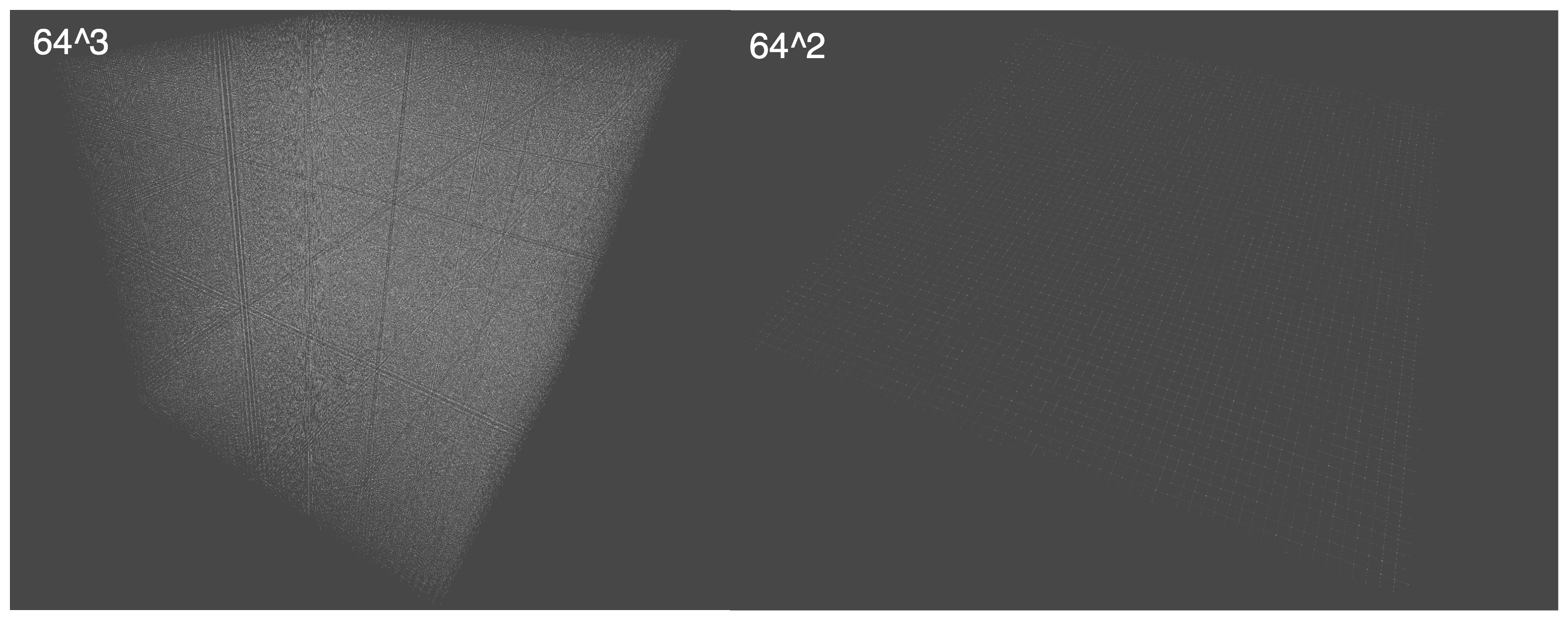
To counteract rapid scaling, a common technique is to downsample the function. Plainly, downsampling is when a lower resolution than the target resolution is resolved/sampled; given a grid of 64 divisions along 3 axises (64^3 points), a downscaling factor of 2 would take only every second point along every axis for 32 divisons, 32^3 points which is smaller by a factor of 8. This is reminiscent of LoD’s, but unlike LoDs, this scaling factor would likely apply to the entire map, as inconsistent downsampling may cause persistent artifacts in resolution disparity, and further solutions to resolve this are probably overkill.
Moreover, purely downsampling a 3D map is unintuitive for our specific use-case. Remember, our goal is to supply dynamic SurfaceHeights and SquashHeights. Putting squash-height to the side, Surface Height is directly correlated to a spatial-axis, if multiple samples along the axis disagree on the surface height, the result may be unpredictable. Now, this may not be undesirable, a 3D-based biome system could support such a sampling strategy, as unintuitive as it is, but in many cases, surfaces are two dimensional(as in not layered) meriting a different approach.
Since Surface & Squash Height are intuitively two dimensional, they should be represented with 2D noise sampling. The most basic advantage is that 2D noise sampling is faster. Simplex noise has a time complexity of O(K^2) where K is the number of dimensions; this is likely an optimistic estimate, as there are likely more complexities with each dimension. Having said that, 2D simplex noise would still be more than 2 times as efficient as 3D. But more importantly, there are far, far less samples necessary. Supposing that this plane is aligned with the XZPlane, all 3D samples of the same xz coordinate would project onto the same 2D sample–effectively collapsing the Y dimension. Ignoring LoDs, for an average sized map of ~640 divisions per axis, the number of samples from 3D to 2D shrinks from 262 million to less than half a million.
With two simple 2D noise function for SurfaceHeight and SquashHeight respectively, the results are barely satisfactory. Since the influence of SquashHeight is sublime, such a method may be alright–but the same cannot be said for SurfaceHeight. As SurfaceHeight strongly determines Surface-features, it becomes evident pretty soon that a single noise map is too repetitive.
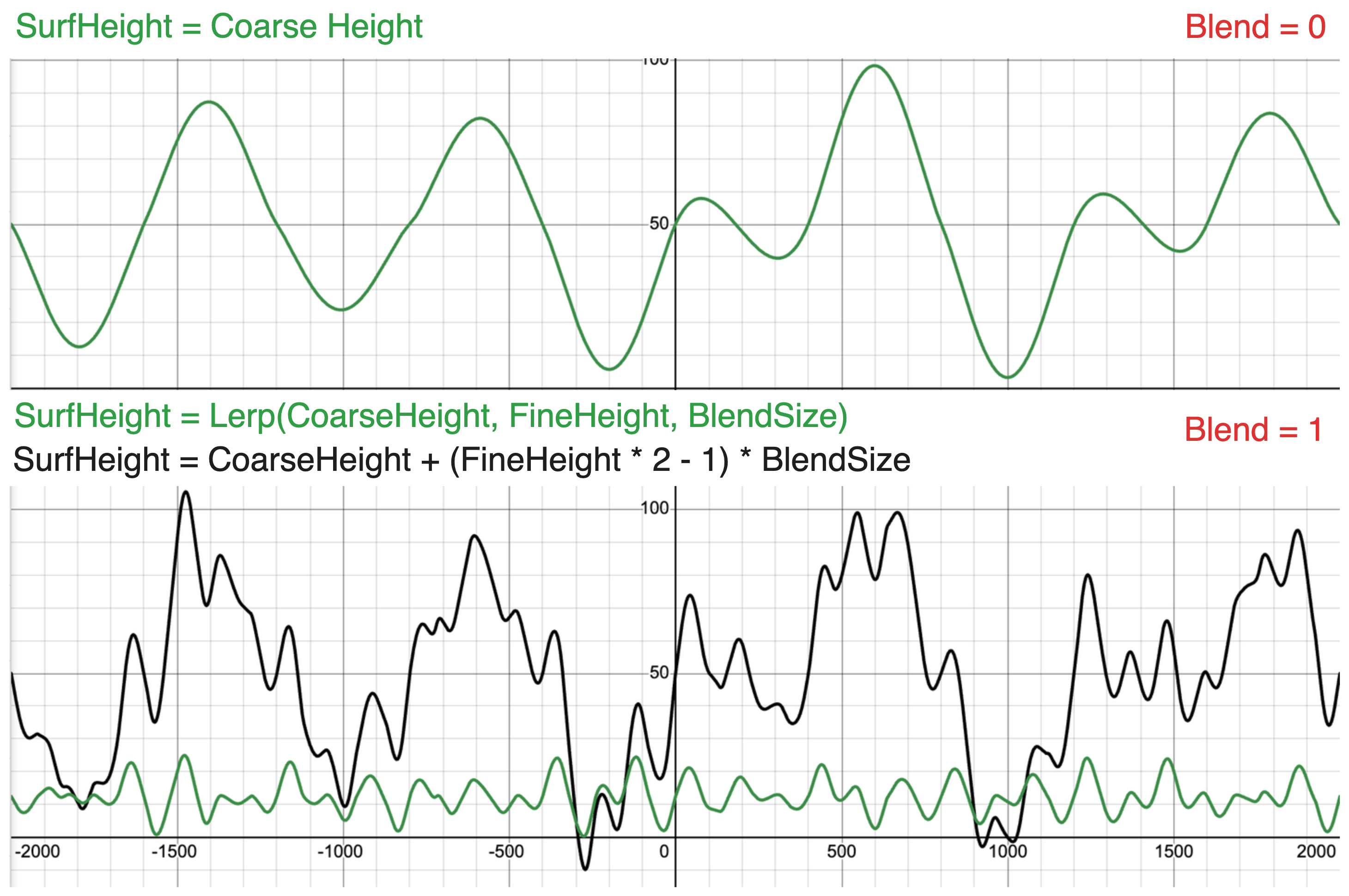
Returning to Henrik’s video, he discusses a way to overcome these challenges through noise map layering. In Minecraft’s case, he lists three noise maps, Continental, Peaks & Valleys, and Erosion which directly contribute to creating the surface map. From what I can gather, erosion here does not refer to actual hydraulic erosion, which is both expensive and requires inter-chunk communication, but a blend factor between Continental & PV(Peaks & Valleys). Giess refers to Continental noise as the general base height for the terrain while PV noise demarcates small scale features(such as peaks and valleys). This type of wording is closely tied to the bezier based interpolation which transforms the noise to create such features; so worded a different way, the three noise maps are CoarseHeight, FineHeight, and BlendSize. The final surface height is defined as such.
SurfaceHeight = lerp(CoarseHeight, FineHeight, BlendSize) = CoarseHeight(1-BlendSize) + FineHeight(BlendSize)
In actuality, this isn’t a direct linear interpolation since doing so treats Coarse and Fine details as equal when it should really be fine detail added ontop of the base height. That way, the terrain still preserves the underlying Coarse shape.
SurfaceHeight = CoarseHeight + (FineHeight * 2 - 1) * BlendSize
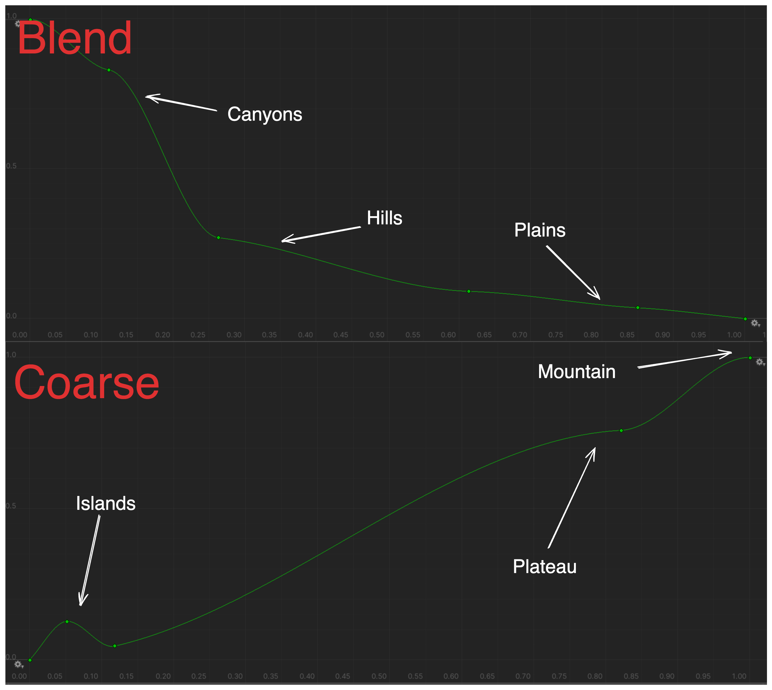
What is more, by defining custom bezier interpolations for each noise function, we can organize surfaces into groups with recognizable features, useful in deciding biomes.
3D Noise
So far, we’ve been relying on a single noise map for cave generation. This works alright, but like SurfaceHeight, it could do with a bit of variety. If one were to try to accomplish this through manipulating an interpolation curve, one would find that all this can control is the frequency of caves; to get windy caves, open caves, and large caves requires the noise itself to be a different shape.
To start, we can use the same technique to layer noise maps to get a variety of sizes. If we define a coarse cave noise function and a fine cave noise function, a third noise map can be defined to control the blend between this coarse and fine map. As these noise maps don’t build ontop of each other(like SurfaceHeight), they may be a direct linear interpolation. Let’s refer to this blend-map as CaveSize.
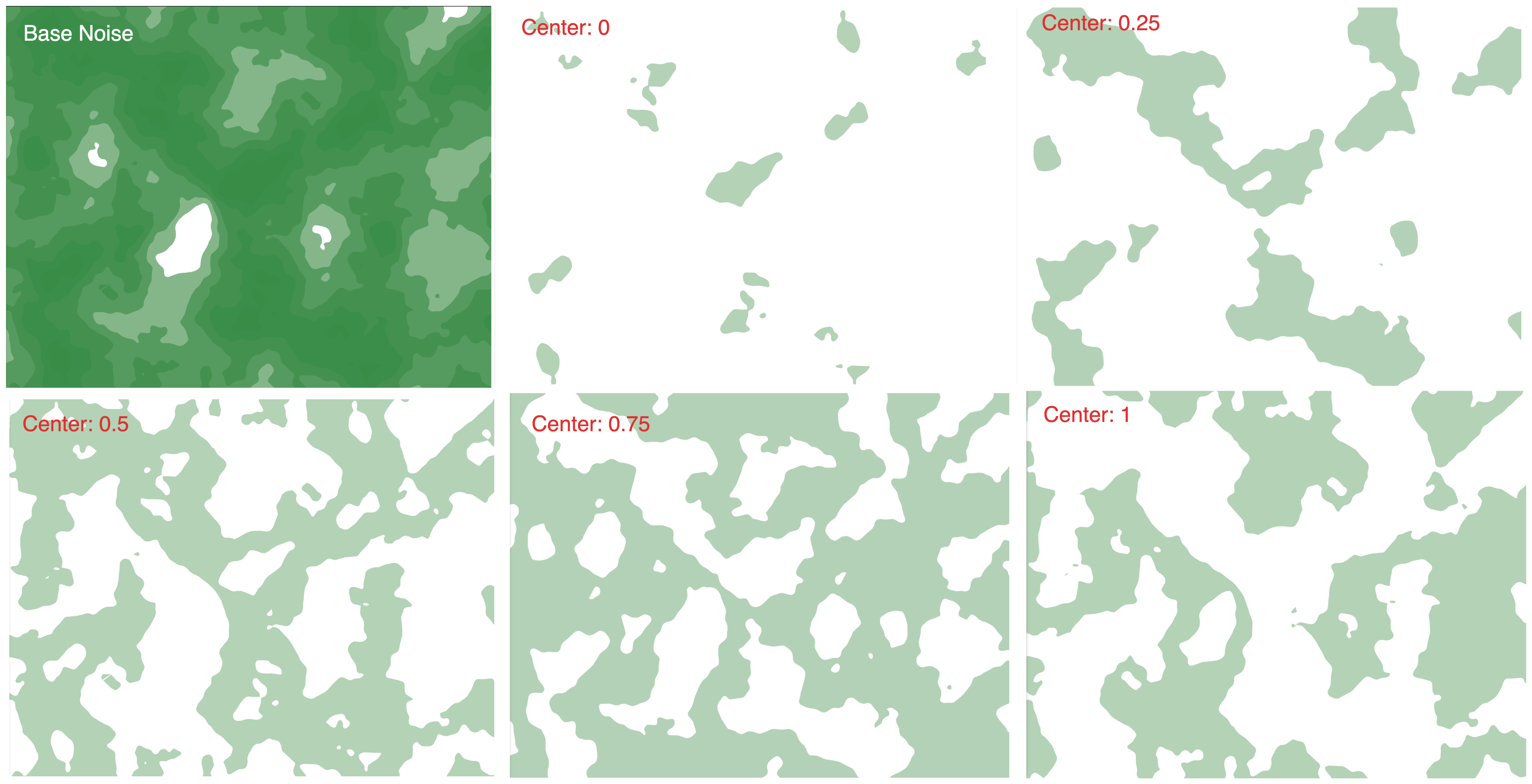
Controlling the shape of caves is harder. Right now caves are… blobular? To create windy caves, we can achieve what we want by figuring out the distance from each point in a cave to the cave wall, and only retaining points adjacent to the cave wall.
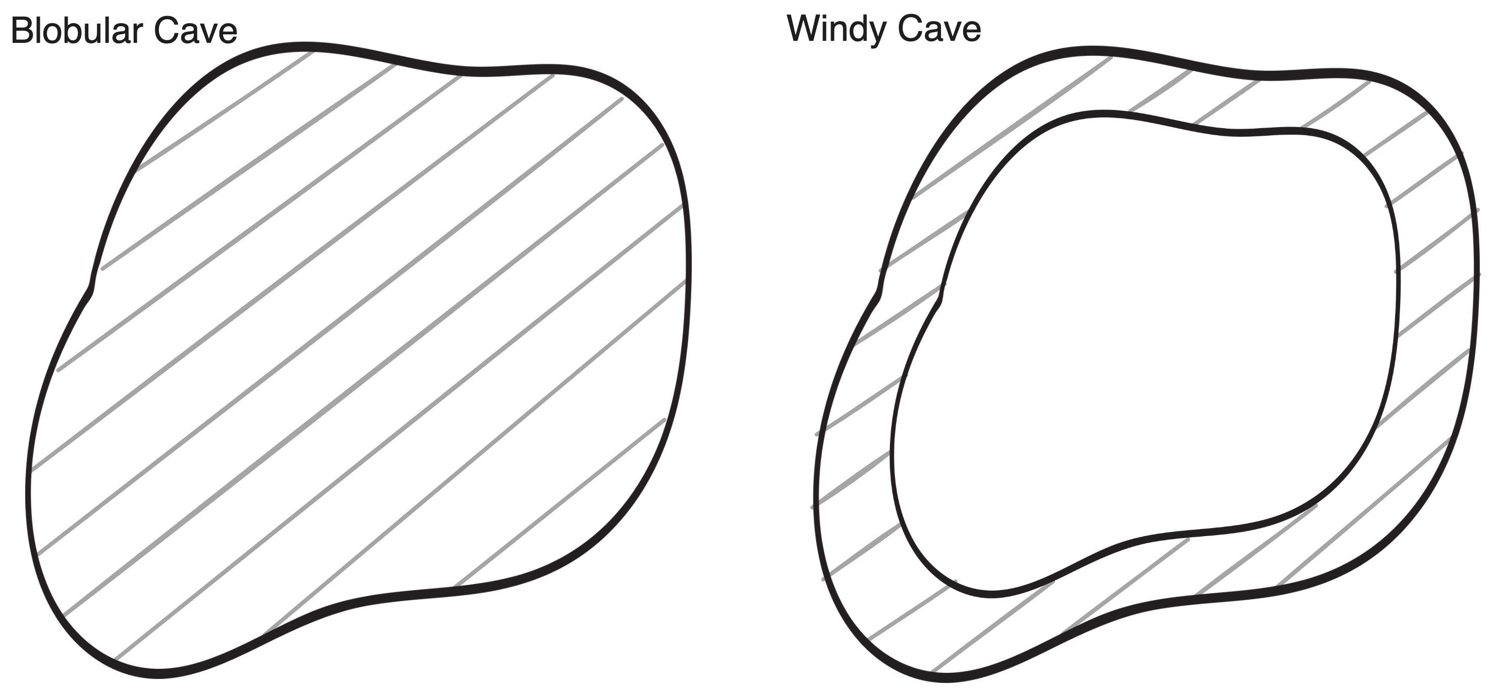
There’s a better way to describe this. If the original noise function’s caves represent areas of lower density, this may be reworded as the cave shape is defined by the distance from each density to zero. Then, to obtain cave generation based on “the distance to the cave wall”, it becomes clear that we need to remeasure each density as the ‘distance to the wall’. Since the cave-wall is a surface, meaning it’s defined by our IsoValue, the distance to the cave wall is just the density difference between each point and the IsoValue. We can call then call our measuring point(IsoValue) the CaveShape.
There’s a bit of nuance with this. Having each density as the distance from 0 means the entire range of density may be utilized given that the range of density is positive. However as soon as our measuring point shifts from one of the endpoints of the range, we are unable to fully utilize the full range of density. For instance, if the original density is a random value in the range [0, 1], by recalculating every density as the distance to 0.5, the range of possible values is now [0, 0.5]. To cover the entire range, we need to remap every distance by the specific range it’s a part of.
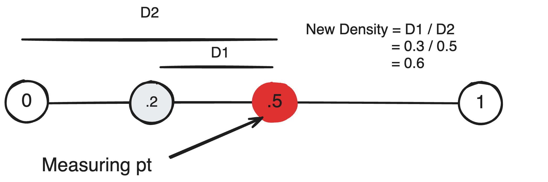
Visually here is what’s happening.
Here is the code equivalent:
1 | GetNoiseCentered(val, center, bottom, top){ |
InverseLerp(a, b, c) = (c - a) / (b - a)
Currently, our way of controlling cave frequency works, but is inconsistent with our other systems. CaveSize and CaveShape are both noise maps while cave frequency still requires us to work with bezier curves. This is even more complicated as CaveSize blends between two noise functions, so the exact cave frequency would also rely on the blend factor between two bezier curves. Furthermore, as biomes should also be able to organize off of cave features, CaveSize and CaveShape would ideally conform to the same sampling method as the other biome-deciding noise functions–that is a 2D map. To remain inline with this model, a 2D map for CaveFrequency should also be defined.
A noise map however returns a single number for every sample which we need to somehow use to control the frequency of cave generation. Luckily, this can be quickly solved through the use of a power function, by raising our density to the power of cave frequency. As cave frequency approaches 1, the slope of this line approaches linear, and as cave frequency approaches 0, the density approaches 1 across the range (-∞, ∞).
Final Cave Function
1 | Noise Maps: 5 |
We subtract CaveBlend from 1 because less caves means more density
Actually, with just CoarseCaveNoise & FineCaveNoise, since we are able to generate seemingly unique noise maps by altering the Size, Shape, and Frequency, such a technique can be used to fake unique noise maps during generation. Particularly, underground materials which should naturally blend into each other may be accomplished through individual unqiue noise functions for every material, then taking the material with the maximum output at each sample. By instead only assigning a size, shape, & frequency for each material, one could achieve the same effect by only sampling two noise maps and reinterpreting every result based on each material’s criteria.
Code Source
Optimized HLSL Parallel Implementation
2DNoise Samples are cached and stored in a surfData
1 |
|