Biomes

 2024/08/10 

Overview

Terrain Generation is a balance between randomness and predictability. Realistic terrain is random, as the many eons of erosion and geological events layered accumulating in natural terrain is dense, so too must the layers of complexity be in mimicking a similar terrain. But realistic terrain is also predictable, for while geological events may be densely accumulated, their individual effects are regional, and so too should terrain possess localized-regional features indicative of regional geolocial activity. Regionality means that nearby terrain generation is naturally similar to each other such that certain features can be predicted based on regional indicators.

Noise-based Terrain Generation can have a similar effect. With one octave on a singular noise function, a vector gradient situated on a simplex corner has a similar effect as a geological feature in as much as exerting a localized influence on nearby terrain. By layering octaves and noise functions, these regional effects can become more pronounced, or rather more varied warranting different names such as “plateau”, “plain”, “hill”. However these names are only superficial, in that the noise functions responsible for these features are not aware of these designations and subsequently not conscious of their presence during or after creation. Going forward, more abstract systems in Terrain Generation(i.e. Structure Placement) might seek to act upon these features thus requiring a non-arbitrary universal system for identifying them.

Background

Revisiting a previous article, I described two methods for additive content generation(generation dependent on other generated content): prescriptive and descriptive. Briefly, prescriptive generation dictates the generation of its dependencies (and therefore occurs prior to its dependencies), while descriptive generation is dictated by its prerequisites (which occurs before it). In context with Biomes, prescriptive generation prescribes the shape of the terrain based on the selected biome while descriptive generation describes the terrain as a specific biome. The specific approach one chooses to Biome Generation is often heavily influenced by the developer’s fundamental understanding of the purpose of Biomes.

Implementing a prescriptive Biome Generator often is done under the pretense that Biomes dictate the geological activity that shapes the terrain. Continuing the analogy of these being noise functions, each biome is free to define its own noise function or even the effects of its noise functions; if a noise function controls erosion, each biome may define a unique erosion function or a unique erosion factor. The ultimate problem is these definitions(Biomes) are discrete, dissimilar to natural erosion which is continuous. Left alone, the terrain along biome-borders becomes disconnected, requiring extensive(and expensive) smoothing algorithms.

Alternatively, a descriptive Biome Generator seeks to classify the terrain into Biomes through a dynamic set of criteria. In the same article, I made an analogy between this strategy and a wardrobe.

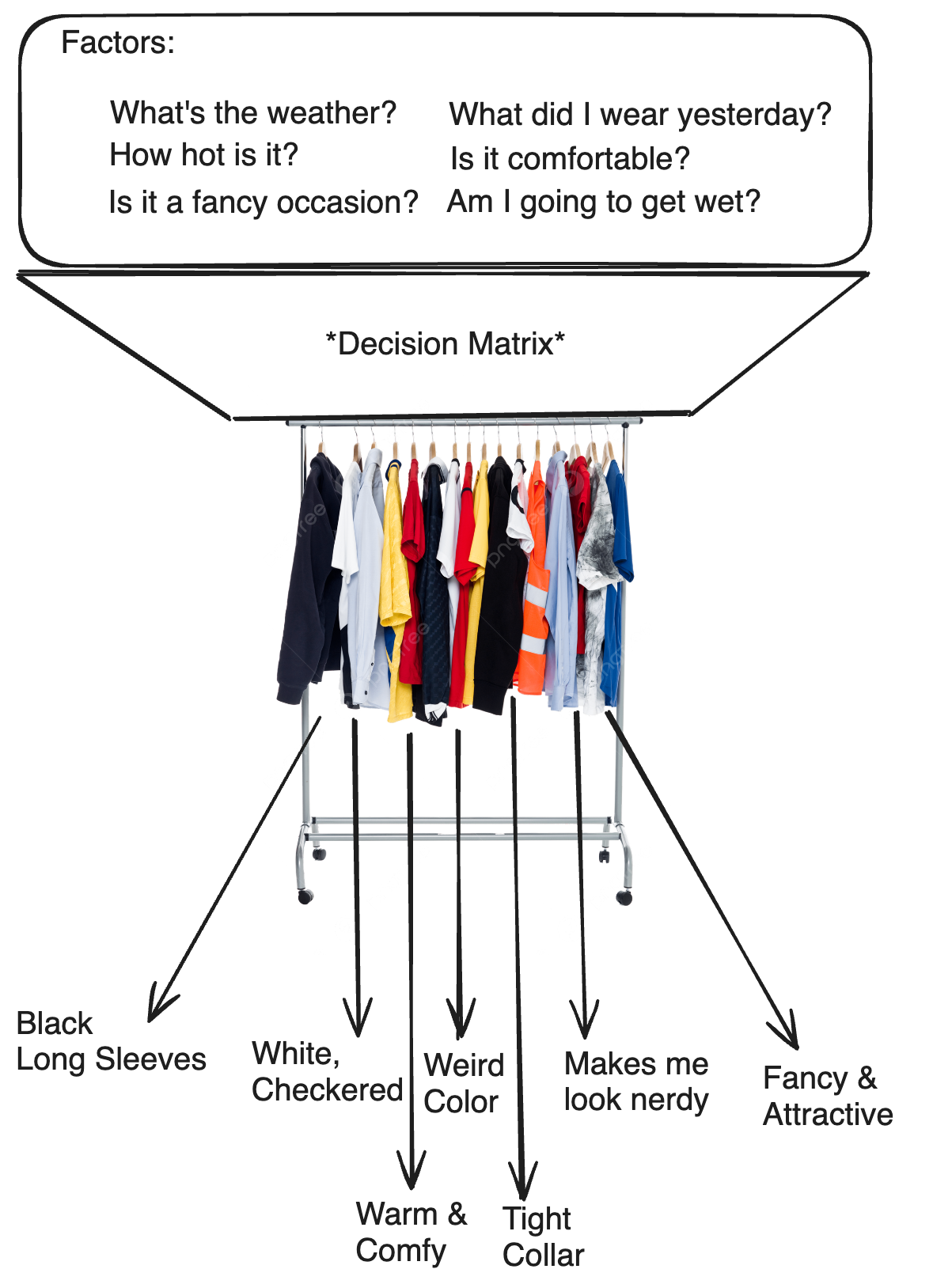
Aspects of generation which directly influence the shape of the terrain are usually features in which preserving continuity is imperative. These aspects are generally the prerequisites by which the decision matrix assignes biomes, thus excluded of the influence of discretized biomes. Contrastingly, aspects which usually involve the apperance of the terrain (structures, materials, animals) are often indifferent to being descritized, and are thus able to take advantage of biome-based organization.

Specifications

When devising ambitous solutions to problems, it helps to keep in mind the limitations in place to decide between different strategies. In this situation, time complexity is perhaps the most egregious out of all terrain generation. In an admittably naiive but common implementation, determining a biome for each grid entry requires each grid entry to verify its conditions against all biomes. With hundreds of millions of grid entries, and a growing number of biomes, this presents a truly daunting task for our computer.

There are ways to counteract this; one could downsample these calculations, but lower resolution usually means choppier biome edges. The problem is that this calculation scales too quickly–with every point and for every new biome. Consquently, while many simple solutions may exist, many find it difficult to overcome this scaling complexity and thus the primary focus of this article will be surmounting this obstacle.

Solution

Returning to the model above, the process of descriptive biome assignment can be subdivided into three portions: the criteria, decision matrix, and output. Given a function, this can be rephrased as defining the input, functionality, and output. In discussing functionality, the output can be seperated using a qualitative identifier, such as a biome index, for the purpose of simplifying the conversation. This biome index can then be used to identify a set of quantitative statistics applied in generation.

Criteria

First and foremost is deciding the Criteria, or input. Previously, when I warned of the time complexity of this task, I actually hid the true severity: the actual time complexity is O(N*M*K), where N is the number of grid entries, M the number of biomes, and K the number of criterions. Given that the goal is to assign a biome that follows our criteria, it is necessary to verify that the biome follows every criterion. Consequently, it is desirable to minimize the number of unique criterions. Simultaneously, a greater amount of criterions allow for greater control over biome placement. Every new criterion adds a new layer of complexity in defining the generation pattern of each biome, expanding variety and faithfulness to natural biomes. Hence, it is also desirable to allow enough criterion to maintain a baseline variety.

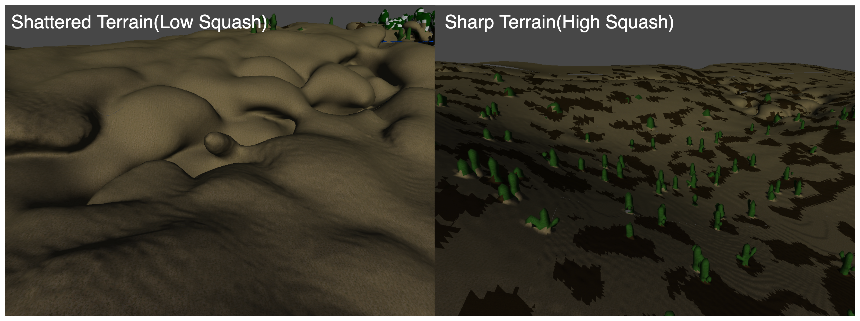
Comparatively, Minecraft‘s generation is (mostly)based off seven such criterion: Continental, Peaks & Valleys, Erosion, Squash, Temperature, Humidity, and Weirdness (In context with last week’s discussion, Continental and PV translates to Coarse and Fine Terrain Height respectively in our implementation). The choice for Coarse/Fine Terrain Height & Erosion is obvious–they directly control the shape of the surface thus allowing biomes to be identified based off terrain-patterns(e.g. plains & mountains). In the same way, Squash Height controls the blend between caves and the surface, responsible for shattered terrain(very broken-up) and sharp terrain(surface is well defined).

The other two maps, Temperature, Humidity & Weirdness, do not contribute to the terrain in any way, but exist to offer variety in biome placement. By their naming scheme, one could take a guess at some of their purposes: temperature could be used to seperate hot and cold biomes so that they(generally) do not generate adjacently; humidity could dictate the difference between deserts & jungles, plains & marshes, etc. All these factors may have little influence on the actual terrain shape, but are arguably even more vital criteria in natural biomes.

Additionally, it is necessary to evaluate the combined terrain height for certain biomes. Specifically, since water is generated relative to the real-world height of the terrain, the only reliable way to identify flooded terrain is through the real combined terrain height. This is the height obtained through Coarse + Erosion * (Fine * 2 - 1). This criterion may also be used to identify beaches and snowy mountain caps. In regards to Terrain-Shape, there are three more factors that influence it that we haven’t discussed thus far: cave shape, cave size and cave frequency. However, these maps aren’t as important as they largely control the underground cave generation while a Biome’s most notable features are usually atop its surface. While they could be completely disregarded, the extremities of these factors may still leave some notable artifacts on the surface.

With that being said, a combined total of 11 criterions is perhaps excessive. Firstly, though Temperature, Humidity & Weirdness offer convenient organization of several similar biomes, they are inherently superficial in as much as they are created solely for biome organization. This means their designations are somewhat arbitrary, in that they could be rearranged with minimal confusion over their influence. For this reason, one could rename Cave Shape, Size & Frequency, which also exert minimal influence over surface generation, to these identifiers. In this way, biomes may maintain the same organization while being able to identify extreme cases of these not-completely arbitrary parameters.

Coarse & Fine Terrain Height are somewhat less arbitrary. As demonstrated by Henrik Kniberg, bezier curves can isolate portions of specific surface generation patterns in either of these maps. However, this is rather nuanced, requiring much fine-tuning to perfect and very project-specific. Moreover, the influence of fine terrain height may even be completely nullified by erosion, and, in all fairness, the scale of detail defined by fine terrain height is too small to be meaningfully considered. Hence, the criteria is reduced into six aspects:

Combined Terrain Height
Erosion
Squash Height
Cave Shape(Temperature)
Cave Size(Humidity)
Cave Frequency(Weirdness)

It’s important to recognize the dimensionality of all these criterions. If you would recall, all the maps listed above are 2D noise functions. As Biomes mostly dictate the aspects of surface(2D) apperance, these conditions are inline with what we expect should influence Biome placement. Fortunately, this also means biome placement can also be 2D, greatly reducing the scale of this operation.

Decision Matrix

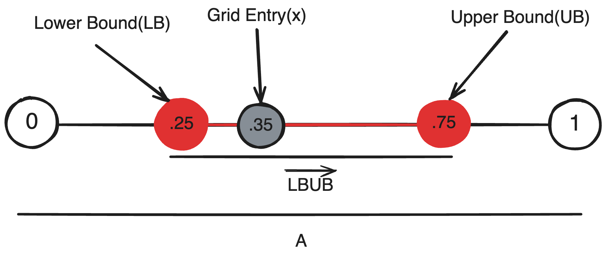
To begin creating a decision matrix, it’s necessary to understand the basis of a decision. That is, how do we decide whether to place a biome at a certain position? Consider a single criterion A that allows us to decide whether a biome ‘fits’ or not. Conceptually, A is a measurement, or a dimension in which every grid entry may yeild a new value {x | x ∈ A}. A simple yet general condition to decide whether a grid entry is part of a Biome is to define a range {LB, UB | (LB ≤ UB) ∩ (UB, LB ∈ A)}, where a grid position is part of a biome if the grid entry is within the range LB ≤ x ≤ UB. Geometrically, we are verifying whether a point lies withing a one-dimensional square, a line segement.

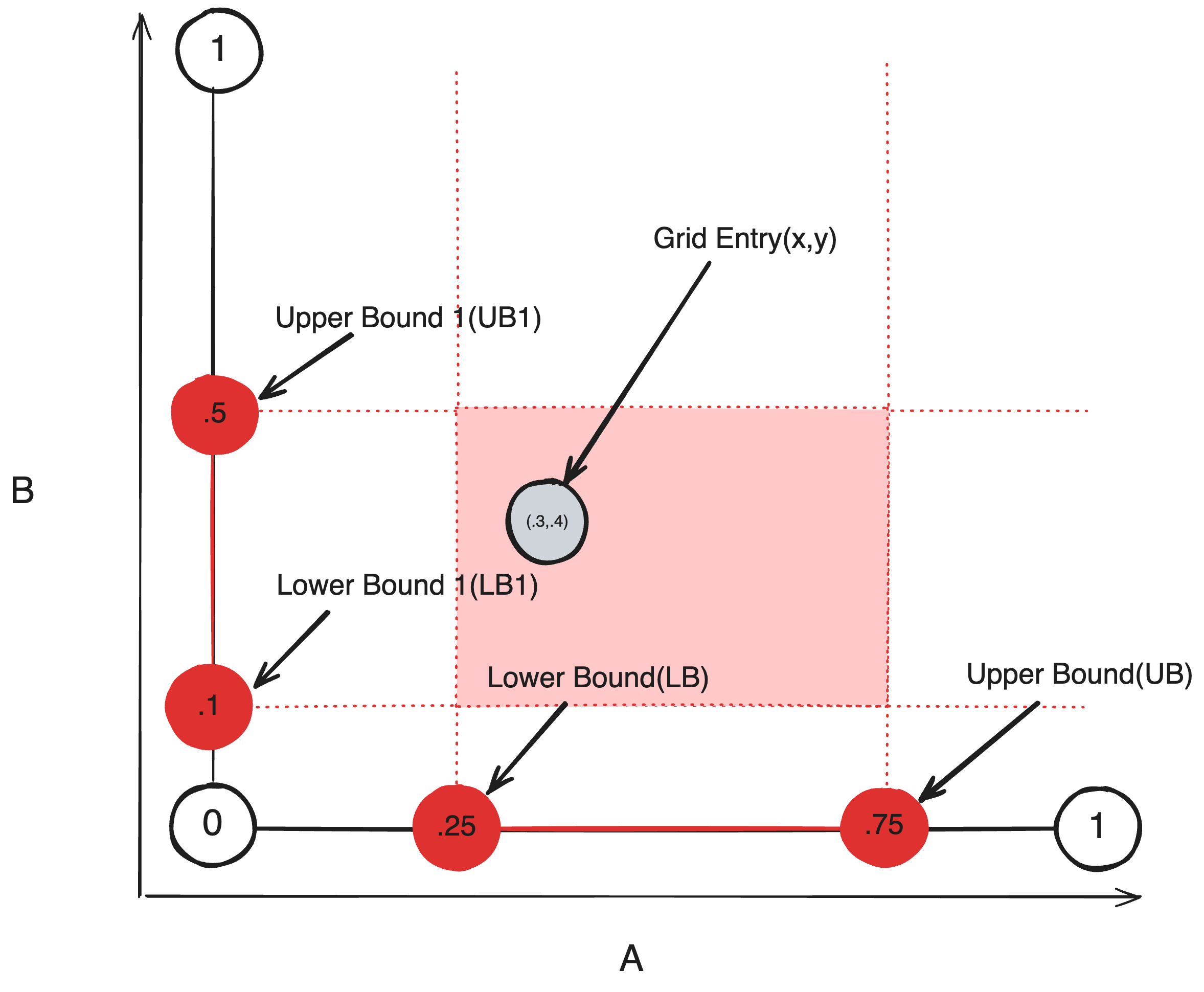
With two criteria, we can extend this definition with a second dimension B. Each grid entry now additionally yeilds a second value {y | y ∈ B}. Additionally we define a new range {LB1, UB1 | (LB1 ≤ UB1) ∩ (UB1, LB1 ∈ B)}; as each grid entry now gives us two values x, y, we can redefine the condition as a grid entry belongs to a biome if and only if both values are within their respective ranges (LB ≤ x ≤ UB) ∩ (LB1 ≤ y ≤ UB1). Geometrically, (x,y) defines a two dimensional coordinate, and the subset of space(AB) where both conditions is true is a square.

Extending for three dimensions and you get the idea.

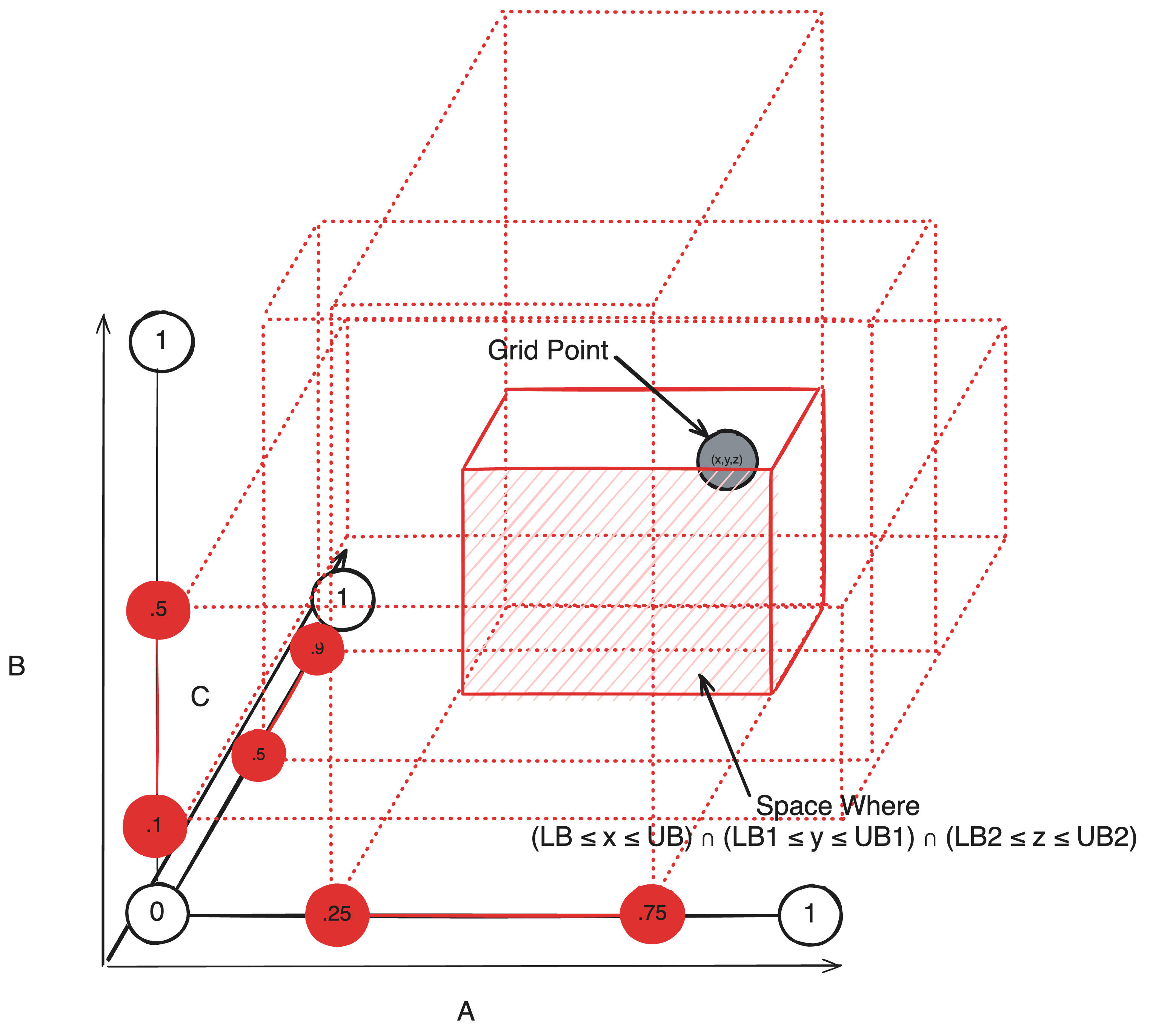
Ultimately, this definition may be generalized in geometrical terms. For any biome, any entry E said to be part of the biome if it satisfies K conditions phrased in the form Π^K_i=0 C_i or (C₀ * C₁ * C₂ … C_K), must also lie within an N-Dimensional Cuboid bounded by (C₀, C₁, C₂ … C_K) where C_i defines the minimum and maximum bound in the i-th dimension of the cuboid. A cuboid like such defines the space for a list of and conditions, but sometimes biomes may appear if one condition or another is true. Luckily, by defining a seperate cuboid, we can account for both cases where either side of any or condition is true. In fact, a better way to do this is to deconstruct any condition into a sum of products, where each term in the expression is a seperate cuboid.

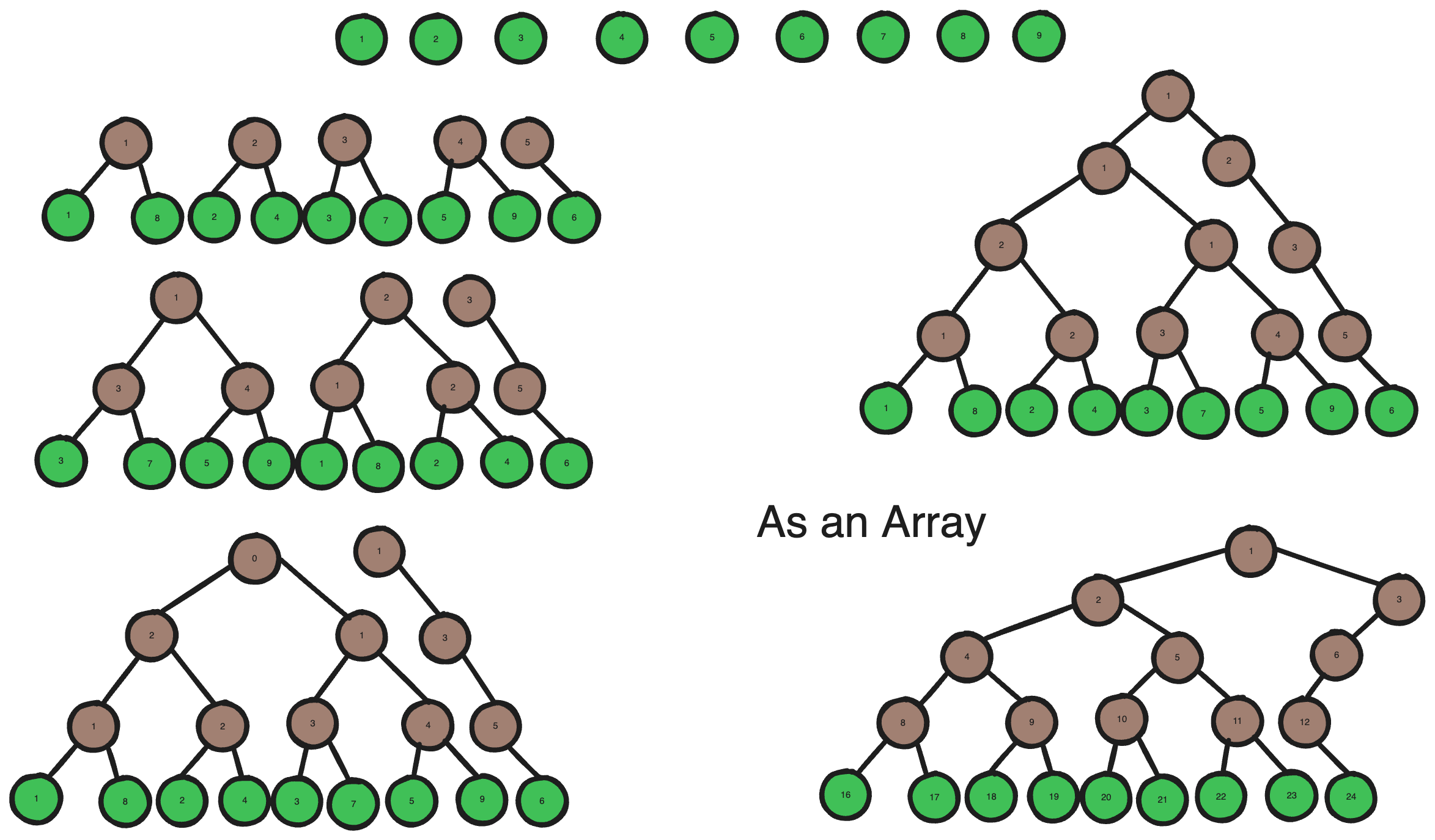
The reason I’ve envisioned the decision matrix in this form is because spatial lookups are a subject of immense study and research. Instead of asking our original question, this representation allows us to ask instead “Which cuboid does a point fall into?”, a query in which many algorithms can expedite. Specifically, a binary R-Tree can reduce the time complexity from O(N*M*K) to O(N*log(M)*K). Long story short, a binary R-Tree is a binary tree where every branch node defines the minimum (K-d)bound that contains both of its children. A parent’s bound is necessarily larger than either of its children, meaning the root node bounds the entire tree; all biome cuboids are leaf nodes and thus determining which biome an entry belongs to requires traversing the tree to find a leaf node that bounds the position.

Construction

It’s first important to clarify that this R-Tree would be a Lookup Table, implying that it is static and will not change during runtime. Barring any odd use-cases, this means that we do not have to worry about insertion or deletion, as the constructed R-Tree shouldn’t need to add or remove biomes. Furthermore, as this tree is static, it only needs to be constructed one-time meaning the time complexity for its construction is practically insignficant; the only meaningful metric should be how fast it can accelerate look-up. I’ll describe a bottom-up strategy for constructing a binary R-Tree in O(M²log(M)).

Initially we are given M leaf nodes, for the first leaf node, search through all other leaf nodes for in which their combined bounding volume is minimized, then pair them together and create a branch node. Do this for every leaf node, and only search through leaf nodes that aren’t paired together. If there is one remaining leaf node, make a branch node solely for it. Then for all the MaxDepth-1 Branch Nodes, repeat the same process to obtain all MaxDepth-2 Branch Nodes. With each ascending level, the amount of branch nodes should approximately half; once there is only one branch node on a level, it is the root node.

Given that this is a balanced binary tree, it can be stored as an array with minimal loss of Space. The standard way to do this is to store the children of node at index i at index 2i and 2i+1 respectively.

Traversal

Traversal of the R-Tree does not differ greatly from a regular R-Tree. As we are querying the bounding biome around a point, a regular traversal involves, for every node we visit, traversal of all children whose bounds contain our point until we reach a leaf node that contains it. Traversing down the tree, we can imagine the bounding box shrinking with every level until we’ve reached a leaf biome. As the tree’s depth is log(M), this ensures a maximum traversal time of O(log(M)) right?

No! Unfortunately, the downside of an R-Tree is that it does not guarantee log time traversal even for a fully balanced tree. This is because while an R-Tree node guarantees that it bounds all children in its subtree, it does not guarantee that all space bounded at a specific tree-depth is bounded uniquely. In other words, though a Node fully contains its children, it cannot guarantee that its children do not overlap. Hence, if a point lies in the bounds of both of a node’s children, it is forced to traverse both children. More troubling is that this problem exists because guaranteeing that both children don’t overlap isn’t even a solvable problem. Take a simple example.

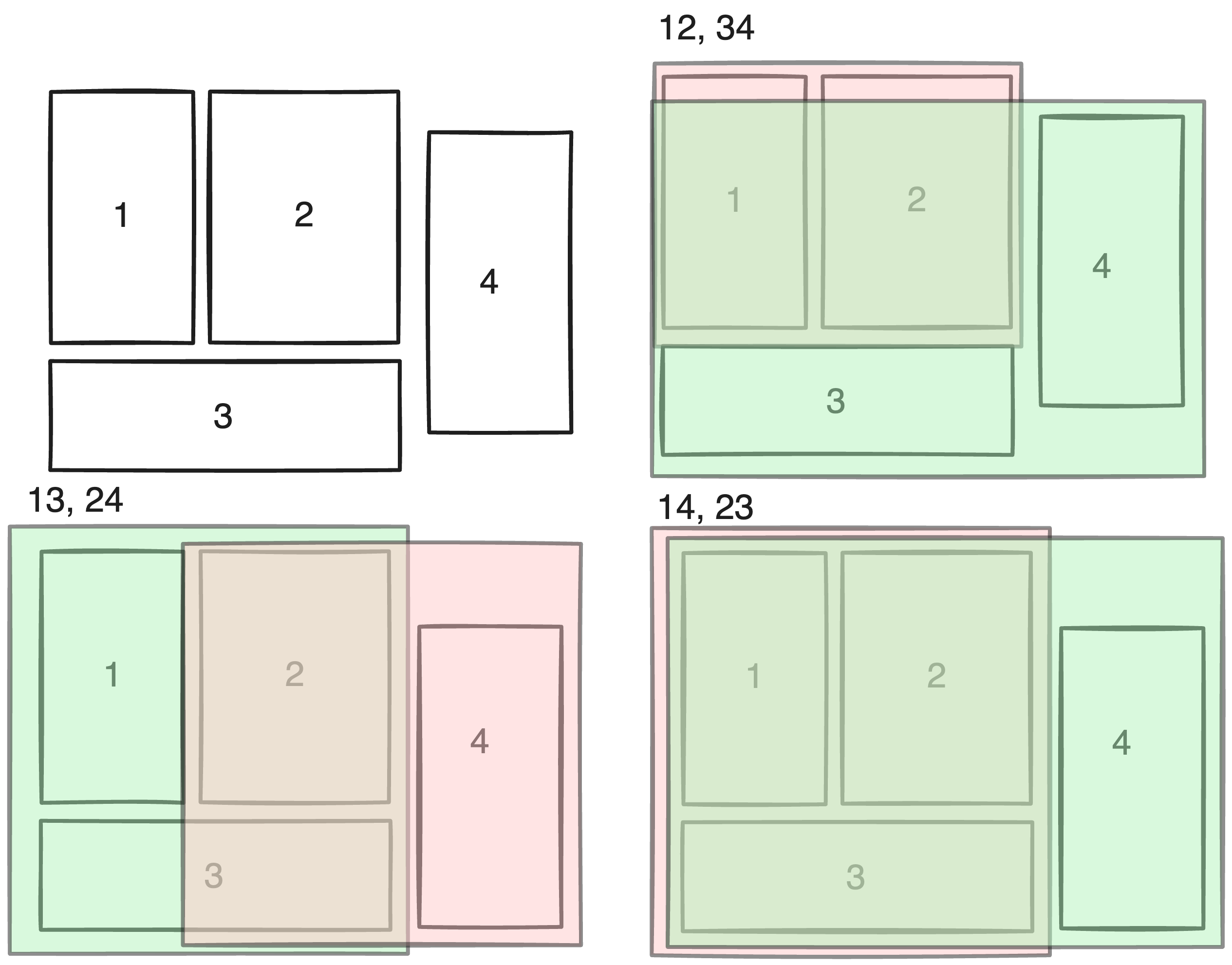
With 4 biomes, a perfectly balanced binary tree should contain 7 nodes; it can do this by creating two groups of 2 leaf nodes, and a single root node to bind both groups. However, it is clear with the example above that no combination of two groups can create fully unique bounds, hence the premise of a balanced R-Tree is that there could be overlap.

This would be okay, traversal of an R-Tree usually involves recursive calls to check both children of every node in case both bound a specific point, except for the fact that shader languages do not allow recursion. Unlike CPU-languages, shader functions don’t actually possess different stack frames, instead all functions are essentially inlined(this owes to the actual hardware differences between CPU and GPU cores). Though this may seem like an implementation detail the lack of recursion is actually really problamatic in this case.

In the case that traversal down a specific path fails(no children contain the point), a recursive call would return to the calling frame, but in our case, we need to manually recreate the calling frame from the child. In a recursive traversal, only a parent can start a recursive call to its child, which means the calling frame for any node is its parent. Obtaining the parent node from the child is simple, if a node’s index is i then its parent is simply floor(i/2).

Having said that, if we just recreate the parent’s conditions from the child, it is no different from calling the parent from the child–which would obviously create an infinite loop as the parent would immediately traverse the child we’re currently at. Instead, the child must also indicate when recreating the parent frame that it has already traversed the current child–but how do we determine which child from the parent’s perspective that is? Easy! If the child is an even number, then it is the first child of its parent, and otherwise, it is the second!

If the parent’s traversal order is first child, second child, then return to its parent, represented as 0, 1, 2 respectively, we can define the following. If a node sees 0, then it knows its parent is starting to traverse it and will try to traverse its first child. If a node sees 1, then it has been returned to by its first child frame and should traverse the second child. If a node sees 2, then it knows it has been returned to by its second child frame and should return to its parent.

In fact, this implementation is even better than the traditional recursive implementation. As the traversal state of the parent can be determined by the child’s index, we don’t need to save the parent’s traversal state when returning from the child. Thus no new stack frames need to be created and memory usage is practically constant as a pose to being limited by the tree depth. This implementation does not have any recursive depth limit.

Code Source

Optimized HLSL Parallel Implementation of Decision Matrix Traversal

struct RNode{
    float minCorner[6];
    float maxCorner[6];
    int biome;
};

StructuredBuffer<RNode> _BiomeRTree;

bool contains(RNode node, float mapData[6]){
    for (int i = 0; i < 6; i++)
    {
        if (mapData[i] < node.minCorner[i] || mapData[i] > node.maxCorner[i])
            return false;
    }
    return true;
}

//No recursion
int GetBiome(float mapData[6]){
    uint curInd = 1;
    uint checkedChild = 0; //0<-unvisited, 1<-visited first child, 2 <- fully visited

    //    if not found     if biome is found
    while(curInd > 0 && _BiomeRTree[curInd-1].biome == -1){

        if(checkedChild == 2){
            checkedChild = curInd % 2 + 1;
            curInd = floor(curInd / 2);
        }
        else if(checkedChild == 0){
            if(contains(_BiomeRTree[curInd * 2 - 1], mapData)){
                curInd = curInd * 2;
                checkedChild = 0;
            }
            else checkedChild = 1;
        }
        else{
            if(contains(_BiomeRTree[curInd * 2], mapData)){
                curInd = curInd * 2 + 1;
                checkedChild = 0;
            }
            else checkedChild = 2;
        }
    }

    return (curInd == 0) ? 0 : _BiomeRTree[curInd-1].biome;
}

C# Construction of Decision Matrix

public class BiomeDictionary
{
    readonly RNode _rTree;

    public int Query(float[] point)
    {
        LeafNode node = QueryNode(_rTree, ref point);
        if (node == null)
            return -1;
        return node.biome;
    }

    public BiomeDictionary(List<Option<BiomeInfo> > biomes)
    {
        List<RNode> leaves = InitializeBiomeRegions(biomes);
        _rTree = ConstructRTree(leaves);
    }

    public RNodeFlat[] FlattenTree()
    {
        int treeSize = GetTreeSize();

        RNodeFlat[] flattenedNodes = new RNodeFlat[treeSize];
        Queue<RNode> treeNodes = new Queue<RNode>();
        treeNodes.Enqueue(_rTree);

        for(int i = 0; i < treeSize; i++)
        {
            RNode cur = treeNodes.Dequeue();
            if(cur == null){
                flattenedNodes[i] = new RNodeFlat(new LeafNode(regionBound.GetNoSpace(6), -1));
                continue;
            }

            flattenedNodes[i] = new RNodeFlat(cur);

            if (cur.GetType() == typeof(LeafNode)) { 
                flattenedNodes[i].biome = ((LeafNode)cur).biome;
                continue;//
            }

            BranchNode branch = (BranchNode)cur;
            treeNodes.Enqueue(branch.childOne);
            treeNodes.Enqueue(branch.childTwo);
        }

        return flattenedNodes;
        //Based on the nature of queues, it will be filled exactly in order of the array
    }
    //
    [System.Runtime.InteropServices.StructLayout(System.Runtime.InteropServices.LayoutKind.Sequential)]
    public struct RNodeFlat
    {
        //Unfortunately, can't use fixed float minCond[6] because unsafe
        //However, this can be redefined into float[6] because it's sequential
        float min_1; float min_2; float min_3; float min_4; float min_5; float min_6;
        float max_1; float max_2; float max_3; float max_4; float max_5; float max_6;
        public int biome; 

        public RNodeFlat(RNode rNode)
        {

            min_1 = rNode.bounds.minCorner[0]; min_2 =  rNode.bounds.minCorner[1]; min_3 = rNode.bounds.minCorner[2];
            min_4 = rNode.bounds.minCorner[3]; min_5 = rNode.bounds.minCorner[4]; min_6 = rNode.bounds.minCorner[5];
            
            max_1 = rNode.bounds.maxCorner[0]; max_2 = rNode.bounds.maxCorner[1]; max_3 = rNode.bounds.maxCorner[2];
            max_4 = rNode.bounds.maxCorner[3]; max_5 = rNode.bounds.maxCorner[4]; max_6 = rNode.bounds.maxCorner[5];

            biome = -1;
        }
    }

    public int GetTreeSize()
    {
        Queue<RNode> treeNodes = new Queue<RNode>();
        treeNodes.Enqueue(_rTree);
        int treeSize = 0;
        while (treeNodes.Count != 0)
        {
            RNode cur = treeNodes.Dequeue();
            treeSize++;

            if(cur == null)
                continue;
            if (cur.GetType() == typeof(LeafNode))
                continue;

            BranchNode branch = (BranchNode)cur;
            treeNodes.Enqueue(branch.childOne);
            treeNodes.Enqueue(branch.childTwo);
        }
        return treeSize;
    }

    LeafNode QueryNode(RNode node, ref float[] point)
    {
        LeafNode OUT = null;
        if (node.GetType() == typeof(LeafNode))
            return (LeafNode)node;

        BranchNode branch = (BranchNode)node;

        if (branch.childOne.bounds.Contains(ref point))
            OUT = QueryNode(branch.childOne, ref point);
        if (OUT == null && branch.childTwo != null && branch.childTwo.bounds.Contains(ref point))
            OUT = QueryNode(branch.childTwo, ref point);

        return OUT;
    }

    RNode ConstructRTree(List<RNode> nodes)
    {
        int nodesInLayer = nodes.Count;
        HashSet<RNode> linked = new HashSet<RNode>();
        List<RNode> ret = new List<RNode>();

        nodes.Sort((RNode a, RNode b) => a.bounds.area.CompareTo(b.bounds.area));

        for (int i = 0; i < nodesInLayer; i++)
        {
            if (linked.Contains(nodes[i]))
                continue;

            BranchNode node = new BranchNode();
            node.bounds = regionBound.GetAllSpace(6);
            node.childOne = nodes[i];
            node.childTwo = null;


            for (int u = i + 1; u < nodesInLayer; u++)
            {
                RNode matchNode = nodes[u];
                if (linked.Contains(matchNode))
                    continue;

                regionBound newRegion = regionBound.mergeRegion(node.childOne.bounds, matchNode.bounds, 6);
                if (newRegion.area <= node.bounds.area)
                {
                    node.bounds = newRegion;
                    node.childTwo = matchNode;
                }
            }
            if (node.childTwo == null)
                node.bounds = node.childOne.bounds;

            ret.Add(node);
            linked.Add(node.childOne);
            linked.Add(node.childTwo);
        }

        if (ret.Count == 1)
            return ret[0];
        return ConstructRTree(ret);
    }

    List<RNode> InitializeBiomeRegions(List<Option<BiomeInfo> > biomes)
    {
        int numOfBiomes = biomes.Count;
        List<RNode> biomeRegions = new List<RNode>();
        for (int i = 0; i < numOfBiomes; i++)
        {
            BiomeInfo.BiomeConditionsData conditions = biomes[i].value.BiomeConditions.value;
            regionBound bounds = new regionBound(6);
            bounds.SetDimensions(conditions);
            bounds.CalculateArea();

            for (int u = i - 1; u >= 0; u--)
            {
                if (RegionIntersects(bounds, biomeRegions[u].bounds, 6))
                    throw new ArgumentException($"Biome {biomes[i].value.name}'s generation intersects with {biomes[u].value.name}");
            }

            biomeRegions.Add(new LeafNode(bounds, i));
        }

        return biomeRegions;
    }

    bool RegionIntersects(regionBound a, regionBound b, int dimensions)
    {
        for (int i = 0; i < dimensions; i++)
        {
            if (a.maxCorner[i] <= b.minCorner[i] || a.minCorner[i] >= b.maxCorner[i])
                return false;
        }
        return true;
    }

    public abstract class RNode
    {
        public regionBound bounds;
    }

    public class BranchNode : RNode
    {
        public RNode childOne; //compiles both leaf and branch nodes
        public RNode childTwo;
    }

    public class LeafNode : RNode
    {
        public int biome;

        public LeafNode(regionBound bounds, int biome)
        {
            this.bounds = bounds;
            this.biome = biome;
        }
    }

    public struct regionBound
    {
        public float[] maxCorner;
        public float[] minCorner;
        public double area;

        public regionBound(int dimensions)
        {
            maxCorner = new float[dimensions];
            minCorner = new float[dimensions];
            area = -1;
        }

        public void SetBoundDimension(int dimension, float min, float max)
        {
            minCorner[dimension] = min;
            maxCorner[dimension] = max;
        }

        public void SetDimensions(BiomeInfo.BiomeConditionsData conditions)
        {
            this.SetBoundDimension(0, conditions.TerrainStart, conditions.TerrainEnd);
            this.SetBoundDimension(1, conditions.ErosionStart, conditions.ErosionEnd);
            this.SetBoundDimension(2, conditions.SquashStart, conditions.SquashEnd);
            this.SetBoundDimension(3, conditions.CaveFreqStart, conditions.CaveFreqEnd);
            this.SetBoundDimension(4, conditions.CaveSizeStart, conditions.CaveSizeEnd);
            this.SetBoundDimension(5, conditions.CaveShapeStart, conditions.CaveShapeEnd);
        }

        public void CalculateArea()
        {
            area = 1;
            for (int i = 0; i < maxCorner.Length; i++)
            {
                area *= maxCorner[i] - minCorner[i];
            }
        }

        public bool Contains(ref float[] point)
        {
            for (int i = 0; i < maxCorner.Length; i++)
            {
                if (point[i] < minCorner[i] || point[i] > maxCorner[i])
                    return false;
            }
            return true;
        }

        public static regionBound mergeRegion(regionBound a, regionBound b, int dimensions)
        {
            regionBound ret = new regionBound(dimensions);
            for (int i = 0; i < dimensions; i++)
            {
                ret.maxCorner[i] = Mathf.Max(a.maxCorner[i], b.maxCorner[i]);
                ret.minCorner[i] = Mathf.Min(a.minCorner[i], b.minCorner[i]);
            }
            ret.CalculateArea();
            return ret;
        }

        public static regionBound GetAllSpace(int dimensions)
        {
            regionBound ret = new regionBound(dimensions);
            for (int i = 0; i < dimensions; i++)
                ret.SetBoundDimension(i, float.MinValue, float.MaxValue);
            ret.area = float.MaxValue;
            return ret;
        }

        public static regionBound GetNoSpace(int dimensions)
        {
            regionBound ret = new regionBound(dimensions);
            for (int i = 0; i < dimensions; i++)
                ret.SetBoundDimension(i, float.MaxValue, float.MinValue);
            ret.area = 0;
            return ret;
        }
    }
}

Author：Jonathan Liu

Link：https://blackmagic919.github.io/AboutMe/2024/08/10/Biomes/

Publish date：August 10th 2024, 9:02:44 pm

Update date：January 17th 2025, 7:35:08 pm

Next Post

Memory Heap
Previous Post

Featured

CATALOG

1. Overview
2. Background
3. Specifications
4. Solution
5. Code Source