Map Representation

 2024/08/31 

Overview

To simulate a realistic dynamic terrain, it is necessary to represent the terrain through an easily accessible and modifiable format. Previously, this was described as a 3D scalar field through which the visible terrain could be loss-lessly recreated through the Marching-Cubes algorithm. The scalar field(referred to as the terrain map or map) provides an efficient way to update and sample the terrain for a variety of purposes including Atmospheric Sampling, Terraforming, Terrain Collision, Pathfinding, Raycasting, etc. Understanding the complexities in its storage and access will be crucial for future articles.

Unlike my usual articles, this one will be instead a collection of ideas and concepts use to aid in efficient storage and access of terrain information for various purposes. Comparatively, these ideas are simpler and the justification for them may vary but all contribute to the purpose of efficient map representation.

Concepts

Data Reproduction

One of the most fundamental concepts in Computer Science is that of Memory Hierarchies and data reproduction. To strike a balance between storage capacity and access speed, this hierarchy expedites computing systems by reducing accesses to slower modules. This can be thought of as a form of caching where a temporary copy of the data is preserved on a higher level where it is more efficiently handled before being copied back to lower levels. In effect this means that many copies of what should be the same object might exist simultaneously.

Ideally, if an object were to have an exact state, an efficient system should first reflect this state in a high level before propogating the change to all copies of the object downwards. Likewise, the object copies should also be updated with progressively lower frequencies descending the heirarchy as it is increasingly more expensive to propogate. Thus a basic theory of memory heirarchies is that latency in an object’s state should increase with access difficulty. But it is arduous envisioning an object as an aggregation of several copies so it is beneficial to define a true state of an object. Usually, this is the top-most memory level(most accessible) since it boasts the lowest update latency meaning it is the most reflective of our ideal state. The top-most level in the above model is a CPU register, which is so fast because it is right next to the processor in a CPU core. For a synchronized single-core process, the register may as well be the true state of an object, but such a definition breaks down for multiprocesser systems.

If a register’s copy of the data were an object’s true state, multiple cores accessing the same object would create multiple copies of the data in their respective registers(and caches) meaning there would be two seperate true states which defeats the purpose of the word’s definition. In such a case, our true state can be the highest level of memory shared by all processors(places responsible for replicating the ideal state): main memory. All higher copies of the data can be envisioned as predictions of immediate futures. But here particularly, this idea is still flawed because(except with unified memory) the GPU also contains its own ‘main memory’ shared by all processors on its chip. Normally, an object is created by and updated by the CPU, so its true state can exist on CPU memory while the GPU maintains a copy purely for visual rendering; the GPU cores do not alter a CPU object’s state so it doesn’t need to access the true copy. However this is not true in our implementation.

The terrain map, a scalar field(object) containing a loss-less representation of the terrain, is first created through a series of GPU commands. It is then stored in the GPU where it is used for visual rendering(Atmosphere), while a CPU command to readback(copy) the map to CPU memory from the stored GPU map is buffered. Further updates to the map then only occur from the CPU which reflects its changes periodically to the GPU’s map. Consequentally while it is being created, the ‘true state’ of the map must exist on the GPU because it is the sole version of the object that exists. But immediately after it is copied to the CPU, the CPU’s copy now becomes the ‘true state’ because all updates are streamlined to that copy first(i.e. lowest latency). Keeping in mind the true state of the map is essential as it determines which direction change should be propogated and which values to trust when copies differ.

A prominent complaint against memory heirarchies is that due to the presence of multiple copies of data, sometimes significant resources are wasted on copies of identical data. This is usually insignificant, but for our terrain map which exists on an extra level(GPU memory) it is enough that effort should be taken to reduce its size.

Unit Compression

From the discussion so far, the terrain can be deconstructed into a scalar field of three values capable of recreating it: density, viscosity, and material, but the question remains: which scalars? The material, which simply points to a seperate LUT entry describing its properties can simply be an integer representing the index in the table. Density and Viscosity both were discussed as a percentage, so an obvious choice would be to represent them using floating-point representation, like a single. This is a tempting choice, but ultimately is an inefficient use of the space.

A single is capable of representing a distribution of numbers from ±3.4×10³⁸ and some special states while an (unsigned)integer is capable of representing integers from ±4.8 * 10⁹. Since both have the same amount of states(32 bits), it should become evident that integer representation has a much finer density of states in its range than float. Floating-point can represent ~2³⁰ states between 0 and 1, but with an uneven distribution near 0 while scaling down integer representation can fit 2³² states with a perfectly even distribution. Moreover for any finite range, integer representation can represent a finer and more even distribution than floating point.

This may seem a bit pedantic, but for lower precision types, representing density and viscosity as integers proves substantially more effective(and simpler) than floating point. 4 bytes is a lot of precision for density; with a decent map resolution, the difference between two consecutive states is so insignificant that it practically doesn’t exist. For this reason, density and viscosity are represented with 1 byte precision allowing for 256 unique states for each(still practically continuous).

Although an even lower precision may be used for density and viscosity, 1 byte division allows for an easy breakup of data. By reducing materials to have 15 bit precision, we can still encode 32k materials(likely more than we’ll ever need), while all three values can fit inside 4 bytes which is conveniently the size of our shader memory management system’s working unit.

The final bit doesn’t have a defined purpose but is very convenient for flags. For instance, this bit is used as a force-marker to indicate not to blend structures in Structure-Placement. Some other purposes it may be used for include the following.

Marking Dirty Modified Terrain
Indicating Meta Data
Marking Selected Terrain

Chunk Size

To enforce efficient procedural generation of terrain, the terrain is usually deconstructed into working chunks which can be independently generated without affecting the integrity of cached(existing) chunks. By extention this also implies that the map, being a direct representation of the terrain, should also be seperable into similar chunks. Note the suffix ‘-able’ means that even though it may not necessaraily be represented in memory as seperate units, it is still able to be divided and read independent of other chunks. Whether it is actually divided is dependent on the use-case and rational related to implementation.

An example of this can be illustrated like so: if the most the viewer can see at most at any single time is 3 chunks away, then the total amount of chunks that can ever be loaded at once is (3+3+1) ^ 3 = 343 chunks. If each chunk is 16^3 = 4096 map units(word/4 bytes), then the most amount of memory that can ever be occupied storing terrain maps is 343 * 4096 = 1,404,928 map units or ~5.6 Mb. While each chunk-map can be stored seperately, if we know that collectively they occupy 5.6 Mb, they can also be combined into an aggregate object of that size. Likewise, we know that if another chunk’s map is created, there must always be enough space freeable in the aggregate object to store it. Thus, though the individual maps are not seperated because they’re collected in one memory location, they are seperable because each chunk map is stored adjacently and addressable within the collective object.

Hence with a seperable model, a chunk-map can be identified as a region of congruent memory. But wait, why is the diameter of the map in the previous diagram 16? Sure if you count the amount of spaces along either dimension you get 16, but this is wrong! Marching Cubes constructs geometry based on samples placed on the corners of a cube. For any 3D subspace divided into a grid of size (i, j, k) where the amount of spaces is i*j*k, the amount of corners is (i+1)*(j+1)*(k+1). So in reality, the diagram depicts a map with a diameter of 17 map entries.

But this creates a problem. The final corner is in fact the first corner of the immediately adjacent chunk. Unlike grid spaces, if map information is stored at grid corners, duplicate corners will be stored by both adjacent chunks which both need to access the data.

In fact, if we’re to stay loyal to the chunk map definition of being a direct representation of the terrain capable of recreating the chunk’s terrain without loss, then the amount of duplicate entries is even more than 17 due to smooth normals. According to an article referenced previously, vertex normals for geometry generated through marching cubes can be determined as the normalized change in density from an entry along each vector of the grid. To determine the normal for a grid-locked parent location of a vertex (i, j, k) involves evaluating the change in density along each vector (i-1,j,k) -> (i+1,j,k), (i,j-1,k) -> (i,j+1,k), and (i,j,k-1) -> (i,j,k+1), which given that the range for i,j and k is [0, 16], indicates that the total data read from each dimension is within the range [-1, 17] or 19 values.

The main problem with storing so many duplicate verticies isn’t necessarily wasted space like most would think. The percentage of values that are so called ‘duplicates’ decreases cubically with the chunk-map size so for any decently sized chunk(32-128 units) the percentage of space that is wasted on copied data is less than 1%. Rather, the main challenge is logistical; duplicated entries should represent the same map data, but the existence of two entries introduces a vulnerability whereby these entries may become desynced such that a conflict may form over the true value of the map. Additionally, it further complicates many systems responsible for updating the map which no longer has the guarantee that a map entry exists in one location.

To address these concerns, each map stores grid entries only equivalent to the amount of grid spaces bounded by it by excluding the region’s maximum adjacent corners which is stored in an adjacent chunk-map. The goes against the seperable map model described previously, but the problems that creates can be addressed through direct hashing.

Direct Hashing

If full seperation of chunk-maps is problematic, the alternative is for map queries to find the entries admist non-congruent memory. With the current criteria, all data relevant to generation of the current chunk’s terrain should be contained within only the immediate 26 adjacent chunks of the current chunks. If these are stored in completely seperate buffers managed by the CPU, one could bind all buffers as seperate resources if DirectX12 were to support it(which it doesn’t). But we have a specialized shader based memeory management system, so if each chunk map is represented as a seperate block in the system, instead 26 integers could be bound specifying the address handle in the address buffer which points to the map.

But since the handle already exists in our shader managed memory, it seems circuitous for the CPU to exist as a middle man connecting the modules. The shader task theoretically has access to all terrain maps but no knowledge of where they are located so it requires the CPU to tell it where he handles are for physically adjacent maps. But if there were to be a way to identify these spatially adjacent maps(i.e. query maps in a shader using spatial information), the shader task could just be provided its own chunk’s spatial information and acquire adjacent information independently. In fact, the ability to query maps spatially on a shader is useful for a variety of chunk-independent effects(atmospheric raymarching).

As a base, let’s define a coordinate space, “Grid Space”, that is grid aligned with our combined map and has a unit-scale that’s exactly scaled to coincide with map-entries at every integer coordinate. Furthermore, let’s imagine a unique coordinate that’s scaled with the size of the chunk map to identify a unique integer coordinate for every handle, or a “Chunk Space”. Finally we can also define a coordinate system to identify the entry’s location within the memory block that is mapped to by the chunk’s map handle, or a “Map Space”.

For positive values, the offset location or “Map Coordinate” within a chunk block can be determined from a Grid Coordinate with a simple modular operation GCoord % mapChunkSize. If chunks are tiled like a grid, and a chunk-map’s origin is situated at the origin of Grid Space, then such a modular operation would return the offset of any grid coordinate to the closest chunk origin below it, which will be the origin of the chunk bounding it. This doesn’t work for negative coordinates however: the remainder operator in hlsl(%) is undefined. A true modulo should return the correct value, and it can be simulated using the formula (x %% n) = (x % n + n) % n. Thus we get the function below.

//C# Hash
int3 MCoord = ((GCoord % mapChunkSize) + mapChunkSize) % mapChunkSize;
//HLSL Hash (Remainder is undefined for negatives)
int3 MCoord = (sign(GCoord) * (abs(GCoord) % mapChunkSize) + mapChunkSize) % mapChunkSize

Now the Chunk Space coordinate of a grid point should be the same for all grid positions mapped to the same point. That is, as long as MCoord is taken relative to the same chunk origin, CCoord(Chunk Space Coordinate) should be the same. Additionally, this form of encoding should be reversable through the formula GCoord = CCoord * mapChunkSize + MCoord. One way this can be found is as CCoord = floor(GCoord/mapChunkSize) using float point arithmetic, but by rearranging the formula above we can get the following formula where all terms evaluate to integers.

1	int3 CCoord = (GCoord - MCoord) / mapChunkSize;

With a unique identifier for all entries within a chunk, and another identifier for the offset within the chunk, the challenge now is to map these into memory. If a map is encoded in memory with a linear encoding scheme, reconstructing the memory offset is very straightforward since we know the map size.

1	int offset = MCoord.x * mapChunkSize * mapChunkSize + MCoord.y * mapChunkSize + MCoord.z;

Since we know the CCoord is directly correlated to a unique map handle, perhaps the worst and most direct solution is to maintain a linked list of nodes, where each node contains a CCoord and memory handle pair indicating the handle for that specific CCoord. To find the map for a grid entry then involves searching through the linked list for the CCoord of the current grid entry to access the memory handle bounded at that node. The logical next step to that train of thought would be a hash map to hash CCoord directly to a location to store the handle.

A dynamic hashmap usually expands over time, rehashing of all its entries as it grows. As discussed previously, it is possible to determine the maximum amount of chunks that can exist at one time which can be used to define a constant sized hash several times this size so that no rehashing is necessary. If a hash conflict is created, the simplest resolution memory-wise is to proceed consecutively down the hash and place it at the next position. Then to identify the chunk between colliding CCoords in queuries, it must also store the raw CCoord as a hash key. All in all with this solution, significant memory would be wasted while worst case time for query and creation of hash entries would remain linear.

The main path to improvement from here relies on one specific fact. To directly hash CCoord without collisions, meaning no remapping is necessary, doesn’t mean CCoord must hash to a unique location for every unique coordinate, but only that the hashed location cannot be occupied by two CCoords at once. If one can guarantee that two maps cannot be created at the same time, there is no need to consider potential collisions between the two hashed CCoords. With this much, I will postulate that a system to directly hash with no collisions to a finite space is possible.

To see why let’s look at an example, let’s look at how offset changes across space.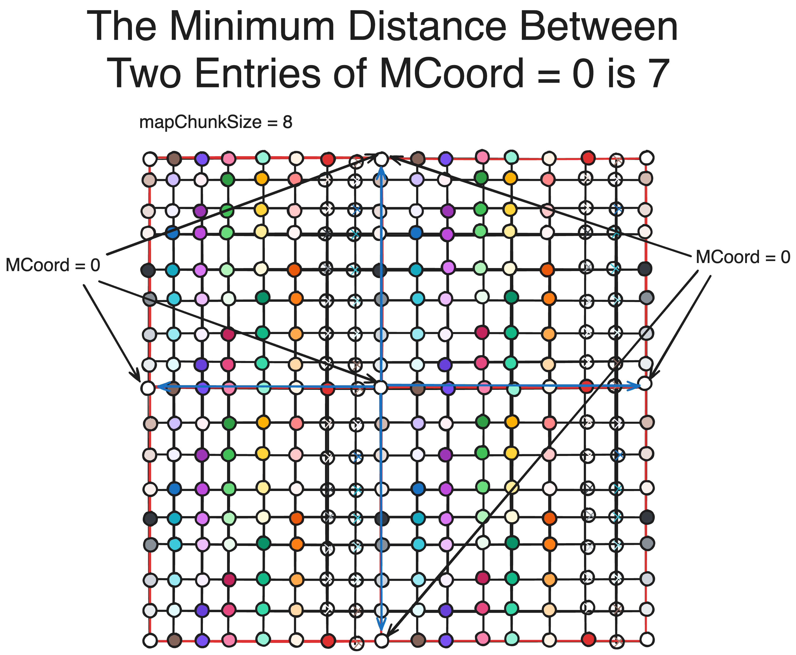

It becomes clear that the minimum distance between two GCoords which map to the same MCoord is mapChunkSize. In the diagram you can see that this property not only exist for the origin, but all points in the map. Additionally, since chunks-maps are loaded from the viewer until a certain distance, there is a maximum physical distance a loaded map must be from another for them to be loaded simultaneously. If we could extend this property for that distance, then we could get a finite colisionless hash.

If the maximum distance from the viewer a map can be to be loaded is N, the total amount of chunks that can be loaded on any axis is 2N+1(see diagram above). If we imagine an origin every 2N+1 integer positions in Chunk Space and get the offset of every CCoord from these origins(the same way MCoord is calculated), we can get a unique offset that is guaranteed to be unique for all chunks that are loaded at any one point in time. Thus, our hashmap for CCoord is simply a copy of the logic for our chunk-map offset.

1
2
3

int numChunksAxis = maxDistChunks * 2 + 1;
int3 HCoord = ((CCoord % numChunksAxis) + numChunksAxis) % numChunksAxis; //Hashed Coord
int hashIndex =  HCoord.x * numChunksAxis * numChunksAxis + HCoord.y * numChunksAxis + HCoord.z;

Another advantage of this system is that it allows for a replacement release strategy, which may be desirable in certain situations. When a chunk-map is created, one can determine the location it hashes to and release the chunk already there(if one exists); that way, a chunk does not need to constantly monitor when it should be released, but will be forcefully released by the chunk replacing it.

Code Source

C# Map Handler

[System.Runtime.InteropServices.StructLayout(System.Runtime.InteropServices.LayoutKind.Sequential)]
public struct MapData
{
    public uint data;

    public bool isDirty{ 
        readonly get => (data & 0x80000000) != 0;
        //Should not edit, but some functions need to
        set => data = value ? data | 0x80000000 : data & 0x7FFFFFFF;
    }

    public int density
    {
        readonly get => (int)data & 0xFF;
        set => data = (data & 0xFFFFFF00) | ((uint)value & 0xFF) | 0x80000000;
    }

    public int viscosity
    {
        readonly get => (int)(data >> 8) & 0xFF;
        set => data = (data & 0xFFFF00FF) | (((uint)value & 0xFF) << 8) | 0x80000000;
    }

    public int material
    {
        readonly get => (int)((data >> 16) & 0x7FFF);
        set => data = (data & 0x8000FFFF) | (uint)((value & 0x7FFF) << 16) | 0x80000000;
    }
}

public static float3 WSToGS(float3 WSPos){return WSPos / lerpScale + mapChunkSize / 2;}
public static float3 GSToWS(float3 GSPos){return (GSPos - mapChunkSize / 2) * lerpScale;}
public static MapData SampleMap(int3 GCoord){
    int3 MCoord = ((GCoord % mapChunkSize) + mapChunkSize) % mapChunkSize;
    int3 CCoord = (GCoord - MCoord) / mapChunkSize;
    int3 HCoord = ((CCoord % numChunksAxis) + numChunksAxis) % numChunksAxis;

    int PIndex = MCoord.x * mapChunkSize * mapChunkSize + MCoord.y * mapChunkSize + MCoord.z;
    int CIndex = HCoord.x * numChunksAxis * numChunksAxis + HCoord.y * numChunksAxis + HCoord.z;
    ChunkMapInfo mapInfo = AddressDict[CIndex];
    //Not available(currently readingback) || Out of Bounds
    if(!mapInfo.valid || math.any(mapInfo.CCoord != CCoord)) 
        return new MapData{data = 4294967295};

    return SectionedMemory[CIndex * numPoints + PIndex];
}

public static int SampleTerrain(int3 GCoord){
    MapData mapData = SampleMap(GCoord);
    return (int)Math.Round(mapData.density * (mapData.viscosity / 255.0f));
}


public struct ChunkMapInfo{
    public int3 CCoord;
    public bool valid;
    public bool isDirty;
}

HLSL Sample GCoord

StructuredBuffer<uint> _MemoryBuffer; //Memory block managed by shader memory manager
StructuredBuffer<uint2> _AddressDict; //Buffered Addresses point into memory block
int3 CCoord;
uint meshSkipInc;
int numCubesPerAxis;

const static int POINT_STRIDE_4BYTE = 1;

uint ReadMapData(int3 coord){
    int3 dCC = floor(coord / (float)numCubesPerAxis);
    coord = abs(dCC * numCubesPerAxis - coord);
    int3 sCCoord = dCC + CCoord;

    uint2 chunkHandle = _AddressDict[HashCoord(sCCoord)];
    if(chunkHandle.x == 0 || chunkHandle.y > meshSkipInc) return 0; 
    else{
    uint chunkResize = meshSkipInc / (float)chunkHandle.y;
    uint address = indexFromCoordManual(coord * chunkResize, numCubesPerAxis * chunkResize) * POINT_STRIDE_4BYTE + chunkHandle.x;

    return _MemoryBuffer[address];
    }
}

Author：Jonathan Liu

Link：https://blackmagic919.github.io/AboutMe/2024/08/31/Map-Representation/

Publish date：August 31st 2024, 7:17:21 pm

Update date：January 17th 2025, 7:35:08 pm

Next Post

Atmospheric Scattering
Previous Post

Memory Heap

CATALOG

1. Overview
2. Concepts
3. Code Source