
Overview
An elegant solution is commonly a simple system that can solve a number of problems. For instance, one may view the cosmos as elegant due to how a few simple laws governing elementary particles can create such complex experiences. Whether these laws are actually ‘simple’ or ‘few’, physicists may disagree, but even so the point stands that we often want to imagine it this way because it somehow feels better that the universe is minimally arbitrary so that all our experience can be derived from an innevitable causality.
This idea applies to any system whereby many problems individually solvable in painstaking case-by-case patches can be unified in a singular solution. Particularly, there are many aspects beneficial, or even indispensible, to modern open-world exploration games that often are resolved through single-purpose solutions. However, aside from being less ‘elegant’ these approaches are tangibly less scalable than a unified generic solutions which may be applicable to situations outside the single-case they were designed to resolve.
But there’s a reason single-purpose solutions exist. Even if physics were destructable to a basic set of particles and instructions, there is no computing system capable of simulating all the interactions necessary to support any meaningful simulation on a macroscopic scale. Single-purpose solutions simplify complex emergent behaviors meaning that they are often much more efficient at their specific task. Simultaneously, unified solutions may need significant optimizations to achieve a similar performance.
Background
To appreciate the ‘elegance’ of atmospheric scattering, it is beneifical that I start by describing the problems it resolves in open-world exploration styled simulations.
One of the best ways to communicate scale in open-worlds is through fog. On still images, it’s difficult to differentiate whether something is small because it’s far away or because it’s physically very small. Similarly, it’s difficult to communicate something very large because it could be confused for being very close to the viewer. A way to overcome this issue is to introduce a fog effect, or a depth-based occlusion that gradually occludes or hazes features based on their distance to the viewer. That way size and distance can be differentiated through ‘fog’, giving depth and scale to large scenes.
In regards to the sky, there are certain expectations that originate from living on a planet like Earth. On earth during daytime, the sky is blue and during the evenings it becomes a brilliant orange fading into a rainbow stretching across the sky. These effects are a direct result of atmospheric scattering, (specifically rayleigh scattering), but are often approximated through skyboxes, which are just textures projected onto an inverted cube/sphere.
On Earth, also commonplace are spatially locked visual effects which we would like to replicate. An example of these are clouds, which occupy fixed locations but are otherwise intangible in that one can simply pass through them with no impedence. Apart from clouds, mist, smoke, and even overlays for water and molten substances can be simulated through custom atmospheric scattering for rays passing through those specific spatial regions.
While all these problems can be individually resolved through aforementioned approaches, in reality they are all an effect of atmospheric light scattering. Atmospheric light scattering is a basic theory on how light interacts with small particles, like gas molecules or water moisture. By staying genuine to the model, a system can simulate situations outside of just the effects listed above in a manner representive of what would occur in reality. For instance, modifications of certain properties could simulate an atmosphere comprising mostly of carbon dioxide, with red skies and blue-tinted sunsets like those found on Mars. Specifically, by extracting atmospheric information directly from our game, more complex effects like arching rainbows, tornadoes, or ash clouds can be recreated through this very same system.
Specifications
Ideally, our game should strive to minimize arbitrarity and maximize interactivity. By arbitrariness I don’t refer to the procedural nature of the system, evidently the initial terrains is arbitrary since it’s defined by some noise system. Rather, I intend to mean that the terrain is arbitrary if the user cannot modify it completely to their preference. Here, arbitrary is used as the antonym of parametrizable, where if a system is mostly hardcoded and unaccessible to the user, it is maximally arbitrary because most of the parameters are ‘arbitrarily set’ by the developer.
In many games, aspects like clouds and atmospheric fog are often arbitrary because they are dictated by the developer and left completely inaccessible to the user. Even if the user were to transform every other aspect of the terrain in a confined region, the sky/clouds would remain an immutable constant limiting the user. This is understandable, because many of the abstractions in standalone solutions to these problems do not offer a way for intuitive immersive modification like that of terrain.
Consequently, one of the biggest accomplishments triumphed by this solution will be overcoming arbitrariness by parameterizing the atmosphere. This is possible because the unified solution that is Atmospheric Scattering is based upon tangible spatial data and therefore can be intuitively parametrized in a way consistent with an immersive terraform-based strategy.
Basis
Camera Ray
At its base, atmospheric light scattering describes how light interactes with particles in the atmosphere. In a rendering system emulating a real-world model, every pixel drawn to the output-texture conceptually represents the light that reaches the pixel’s position on the camera’s frustrum. There’s a slight caveat with this–considering only the maximum light reaching every position causes most scenes to become a blinding white–and the reason for this is because such a model is not representitve of how our eyes function.
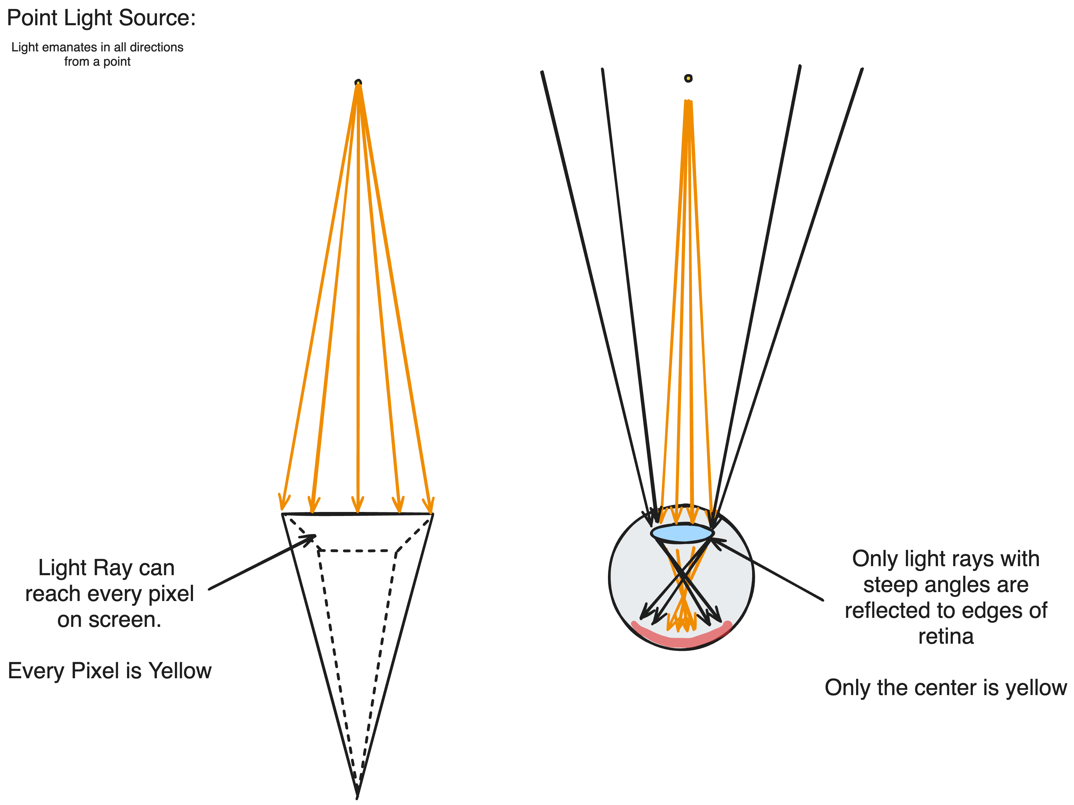
Our eyes possess a lens that focus light onto a retina through which we percieve the world. If we envision the retina as our screen, the reason why light from a light source does not reach every retinal cone is because the lens concentrates rays from the sun spread out across the lens onto a small surface on the retina–allowing rays not from the sun(with a steeper angle) to reach the retina. For this reason, light interactions will be calculated along the camera ray(the ray from the camera origin to the pixel on the frustrum in 3D space), as this represents the light that would be refracted to the pixel’s position in a human eye.
The same way light can reflect off a surface, light can reflect off atmospheric particles into the camera. For that reflected light to reach our retinal cone, it must be reflected by a particle along the camera ray of the pixel representing the cone. In a saturated atmosphere, multiple particles could lie on that single ray in which case the total light reaching our pixel should be the sum of all light reflected off every particle on the ray. On a continuous ray, this can be represented as the integral of in-scattered light(light scattered onto the ray) evaluated along the ray. In Accurate Atmosphere Scattering, an nvidia GPU gem article, Sean O’Neil writes this integral below.
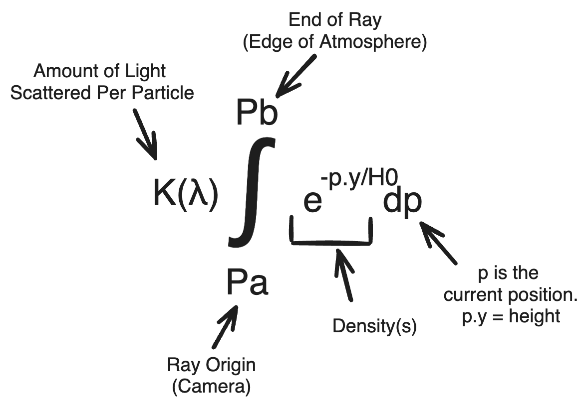
K(λ) in the diagram above symbolizes the reflection coefficient for a given wavelenth λ. If we suppose that the atmosphere comprises of a uniform mixture, the in-scatter coefficient(K) of any single particle should not change across the atmosphere, thus it can be factored out of the integral. Since the solution to the integral of density represents the total mass(amount of particles) along the ray, this expression can be rephrased to mean that the total amount of light reaching the camera is equivalent to the light scattered by a single particle multiplied by the amount of particles along the camera ray.
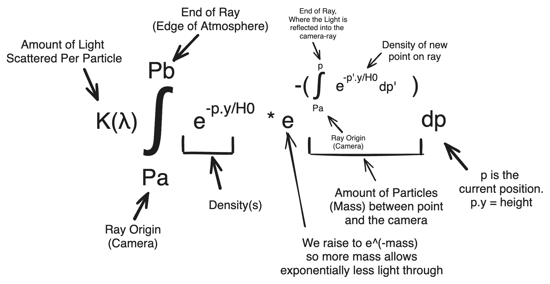
However, since light can be scattered into the camera ray, logically it should also be able to be scattered out of the camera ray. Furthermore, the chance of being reflected out should not be consistent for every photon traveling to the camera–photons reflected into the camera further which travel through more particles should have a higher chance of being reflected. Really, the chance of being reflected away from the camera for a photon traveling along the camera ray to the camera should be proportional to the amount of mass between it and the camera.
Sun Ray
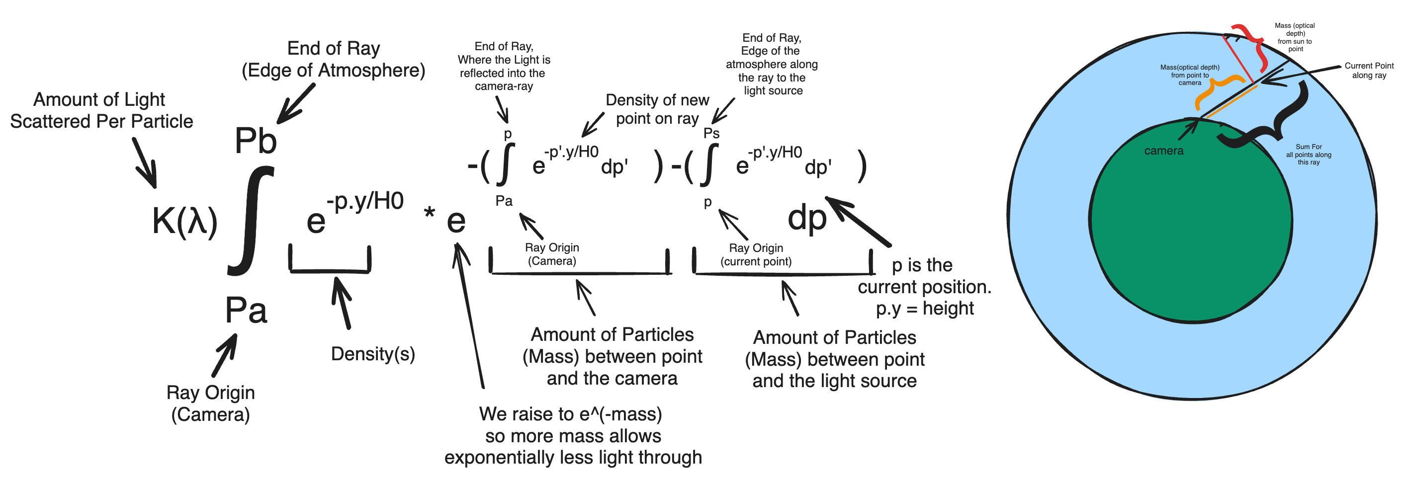
As if this function isn’t complicated enough, we’re still making a fatal assumption: that the amount of light reaching every point along our camera ray is equal. We can start by assuming that all light entering the atmosphere is identical(same wavelengths and amplitudes). Given that this is the case, to be reflected at a certain point into the camera ray, light must first travel from the edge of the atmosphere to the point. Admittedly this light could theoretically come from any direction, but in practice it is a good approximation to only consider the light from the ray going from the point directly to the light source.
As discussed previously, when light travels along a ray to a point, a percentage of light will be reflected out of the ray proportional to the total mass along the ray it is traveling on. By the same principle, light traveling from the edge of the atmosphere to the point at which it’s reflected into the camera ray will be proportionally out-scattered(scattered away from that ray) and be lost in the atmosphere. We can account for this with yet another integral describing the density along this new ray.
Coefficients
Now there are two main forms of atmospheric light scattering many people know, Rayleigh and Mie, which groups different particles by what wavelengths are reflect light in which different directions. While there may be exact physical definitions for these groups, many of their properties can be explained intuitively by extrapolating Rayleigh as representing small opaque particles(dust/molecules), and Mie representing large translucent ones(mist/water).
Different wavelengths of light are scattered differently by particles between of these two groups. Rayleigh scattering scatters higher wavelength light like violet and blue more than lower wavelengths like orange and red which explains blue skies(blue is more likely scattered into the camera ray), and red sunsets(red is less likely to be scattered out of the camera ray). Mie scattering, however scatters both to a relatively similar level, creating mostly misty/foggy scenes like humid jungles. On the basis that Mie particles are usually larger than Rayleigh, this ‘kind-of’ makes sense because small particles may be hit more frequently by photons ocilating at a higher frequency, if one were to envision them as particles, but for larger particles it doesn’t make much of a difference. A visual diagram showing this can be found in Coding Adventures: Atmosphere by Sebastian Lague.
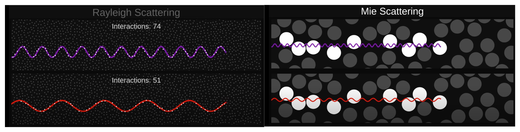
Sebastian Lague: Coding Adventures-Atmosphere. You can see for small particles, higher wavelengths intersect more particles but for larger particles it makes little difference.
Another difference between the two groups is the direction light is reflected off the particles. When light passes between mediums, a portion of light is transmitted, a portion is absorbed, and a portion is reflected; this much is a fundamental basis in optics. For small opaque particles in Rayleigh, much of the light is reflected, but a large portion is also transmitted because it is so small-like shining a light through a thin piece of paper, a significant portion of the light is reflected but another leaks through to the other side. Meanwhile for large translucent particles for Mie, most of the light is transmitted(becuase it’s transparent) while minimal light is reflected and goes in any other direction.
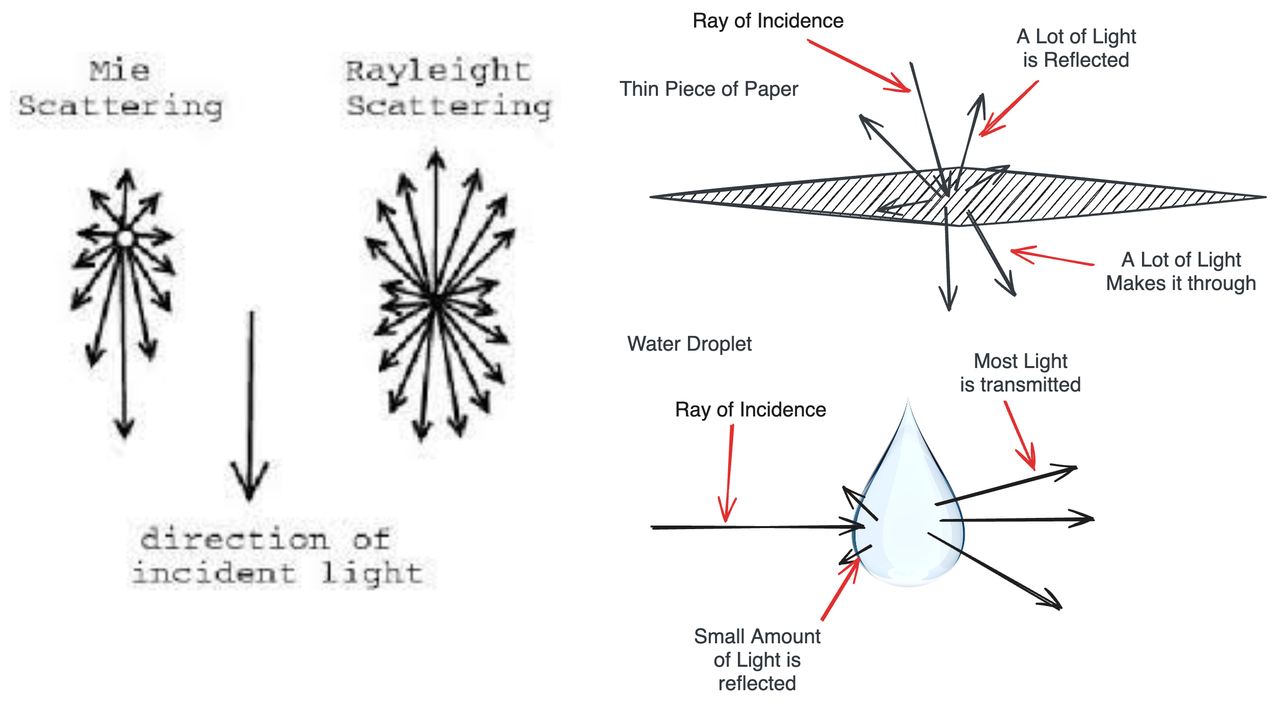
Forgive me physicists if this is not how it actually works. It’s a good enough abstraction to get the point across
What this means is that in discussing atmospheres comprising of these two groups of particles, each group will have unique Scattering Coefficients, K(λ), and a unique directional based coefficient, also known as a phase function, F(θ) where θ is the angle of incidence for a light-ray coming from the light-source reflecting into the camera ray. To simplify things, we will only be considering direction light-sources which means θ is constant across the outer-integral allowing us to factor it out as well.
Final Function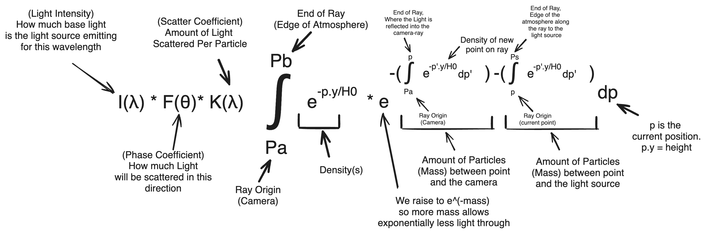
Technically the angle of incidence will be different(always 180 deg) for light on the ray from the edge of the atmosphere to the point of incidence. So you can factor that in to the third integral if you wish.
Acceleration
With the goal of our atmospheric light scattering defined, the next step is figuring out how to implement it as a processable function. For every pixel on our screen, we can calculate the scatter and phase coefficients easily given that we know the camera ray to the pixel. The real challenge here is figuring out what to do with the nested integrals that is the remaining part of the expression.
Usually if integrals cannot be solved beforehand either because the variable of integration changes or the bounds do, the only other option is to approximate the integral using discrete segments. This is true in our case because the camera position and direction can change during runtime, meaning we’ll have unique camera rays for every pixel intergrated for a new region of space. I, and most implementations, use the rectangular rule to approximate the nested integrals because the extra calculations for the trapezoid rule and other strategies do not justify their difference in accuracy.
Unfortunately, this is extremely inefficient because to achieve an acceptable accuracy requires many discrete sample regions, and every region itself must additionally approximate two more integrals for the camera ray and the ray to the light source. And this has to be done for every pixel amongst up to a million pixels in modern screens.
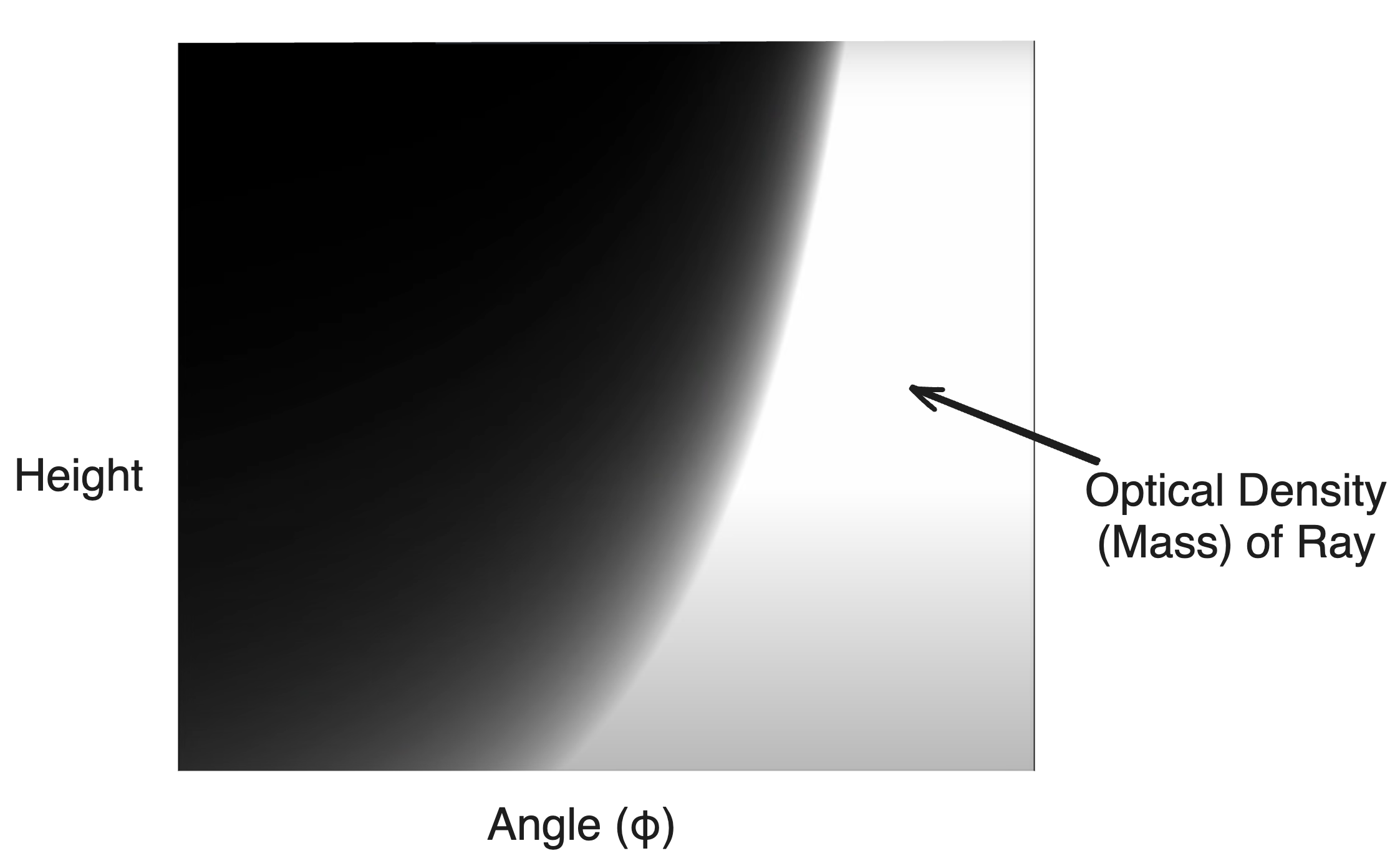
Actually, in his article, Sean O’Niel points out an extreme optimization that can be made with the way he’s defined density(e-h/H0). Since density is a direct function of height, the density will evaluate identically for any two points in the atmosphere of the same height. This means that the ray could sample density on the opposite side of the planet at the same height and achieve the same answer. What’s more, Sean realized that all rays at an identical height on the atmosphere that have the same angle φ, where φ is the angle between the ray and the line perpendicular to the planet’s surface and intersects the position, are indistinguishable from each other with respect to the integrals. What he’s implying is that the solution for the integrals, or the amount of particles/mass, along any ray with identical φ and height will be the same.
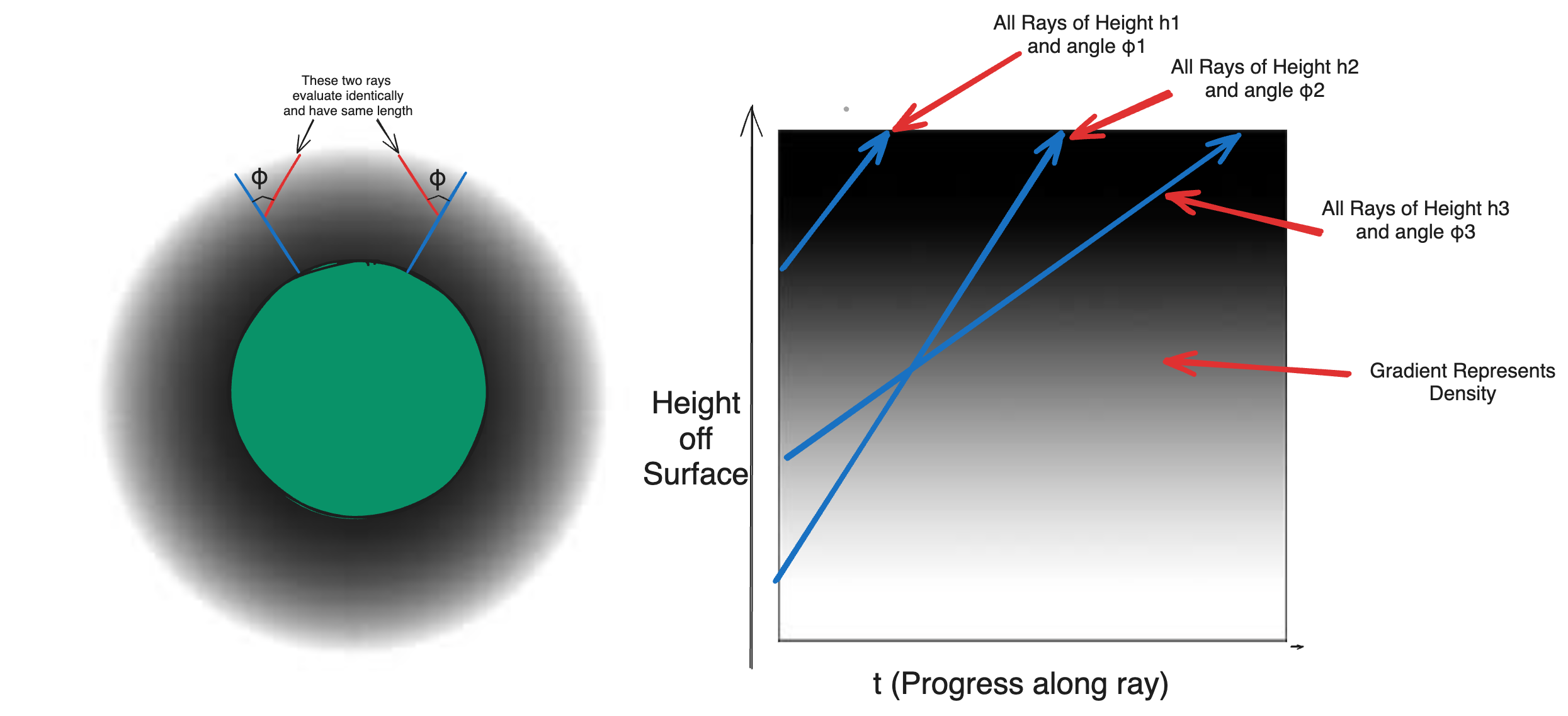
This works because density is a direct function of height, and different angles simply describe a unique line that traverses the gradient. Two rays starting at the same height and with the same angle will essentially traverse the density gradient in the exact same way starting from the same point. The importance of this is that this allows us to precompute a 2D LUT where one dimension is the height off the surface, and the other is the angle of the ray with respect to the perpendicular. Such a LUT could reduce all three integrals into a single lookup.
Credit: Sebastian Lague - Coding Adventures: Atmosphere
Light Rays
A particularly awe-inspiring effect(in my opinion), light rays, also known as god rays, specular rays, sunbeams and crepuscular rays, are shafts of light particularly visible on misty days with the light source partially obstructed with respect to the viewer. In nature, this obstruction normally takes the form of trees or clouds, but physically it could take the form of any semi-opaque object. Visually, light rays are a great way of demonstrating the nature of atmospheric light scattering in a stark and well defined manner.
Previously, I noted that the conditions for light rays were a misty atmosphere because these conditions maximize the effects of atmospheric light scattering over the same volume of atmosphere. This accentuates a light ray by increasing the amount of light reflected across the ray as compared to an obstructed ray through the atmosphere which reflects no light. In the same way, looking parallel to the light-source also boldens these effects as a longer portion of the camera-ray is illuminated by comparison.
In fact, the reason light rays exist is because of a possibility we ignored in discussing the sun ray: that the sun-ray itself could be obstructed. To calculate the amount of light reaching a point along the camera ray, an approximation was attained by falling-off the base light proportional to the mass along a ray traveling directly to the light source, but if this ray were to be obstructed, then no light should be able to reach our point. Likewise the equivalent region on the camera ray should contribute no reflected light, since no light can reach the region in the first place.
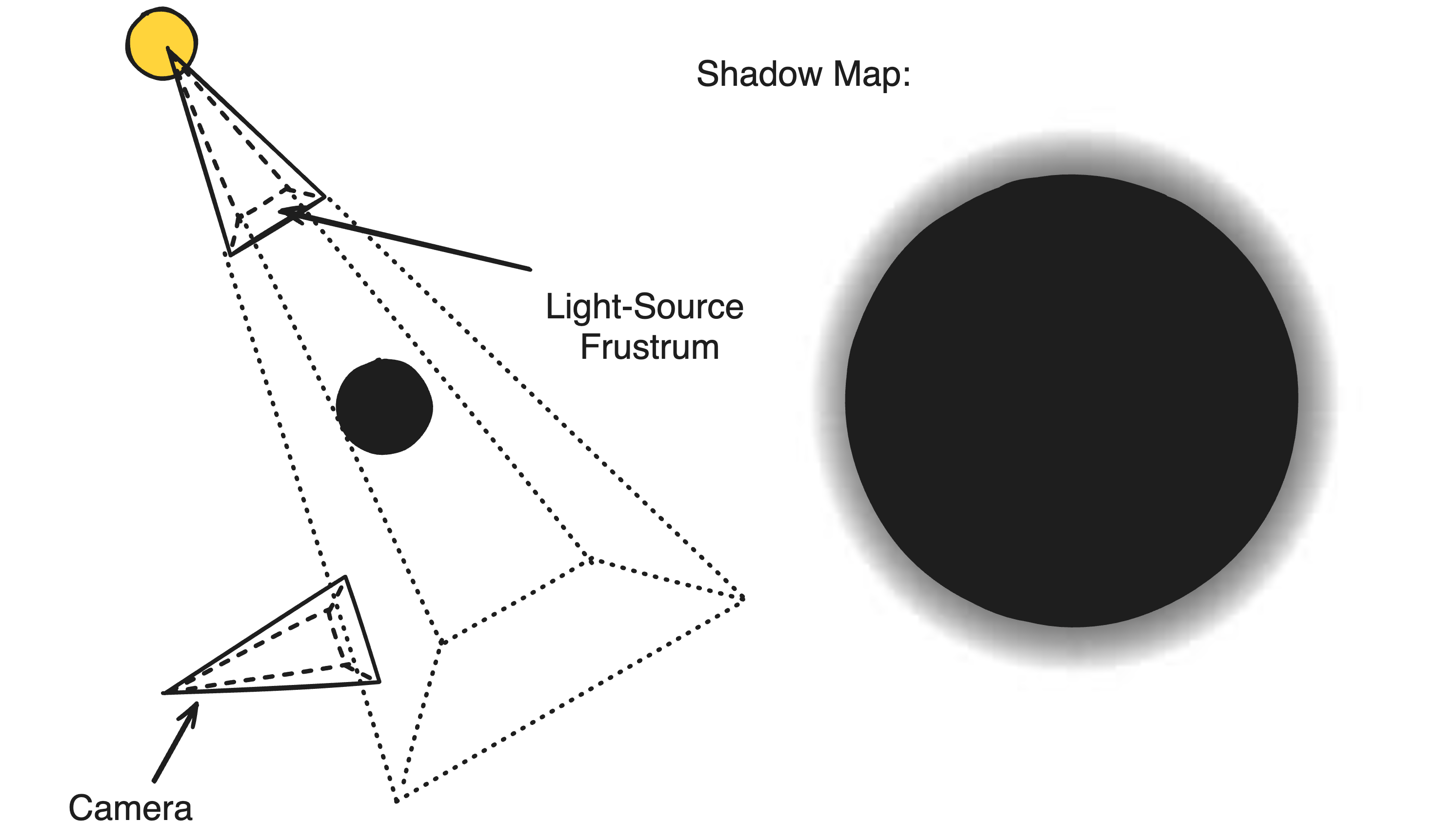
A simple way to determine whether a sun-ray is obstructed is to use what many graphic pipelines refer to as a shadow map, which is basically a depth map drawn around the camera from the perspective of the light source. The depth in question is the depth from the light-source, or the distance from the light-source of the first obstructing surface at every pixel. One can use this to determine whether a position is obstructed(or ‘in shadow’) by determining its distance from the light-source frustrum, then projecting itself onto the frustrum and comparing its distance with the depth of the pixel it is projected onto. Intuitively, if the distance is greater than the distance to the first obstructed surface, then the position must be ‘in-shadow’.
Of course, many optimizations can produce similar effects for a fraction of the speed. One method I’ve read about proposes epipolarly sampling the light-occlusion as light rays spread radially from the light source on the camera screen. Another attempts speed up raymarching by locating all the occlusive regions along a ray through a binary min-max tree. However, these methods usually tradeoff simulation accuracy for their speed.
Extinction
Finally, we have to figure out what to do with the original color of the pixel: the color of the opaque surface originally reflected. According to our logic, the light reflected by other original surface needs to travel through the atmosphere to reach the camera during which a fraction of it will be reflected out of the camera ray. The portion scattered away from the camera is proportional to the mass between the surface and the camera, which we can calculate with our original integral. For finer control, we can also add a scattering coefficient for the surface, in case we want the surface to be more pronounced than the atmosphere.
The astute may have noticed an oversight with this method, the original color of the pixel, the light reflected by the surface, was calculated independent of the atmosphere meaning the light ray managed to reach the surface unimpeded. Technically, if the surface was in the atmosphere this color would be inaccurate, as it fails to account for the portion of light lost from the edge of the atmosphere to the surface. This is a valid point, but in most applications the visual effect is minimal so apart from simulations demanding extreme accuracy, this factor is ignored.
1 | Ip' = Iv + Ip * Ke(λ) x exp(-∫(PaPb)); |
So at long last, we arrive at a beautiful visual atmosphere.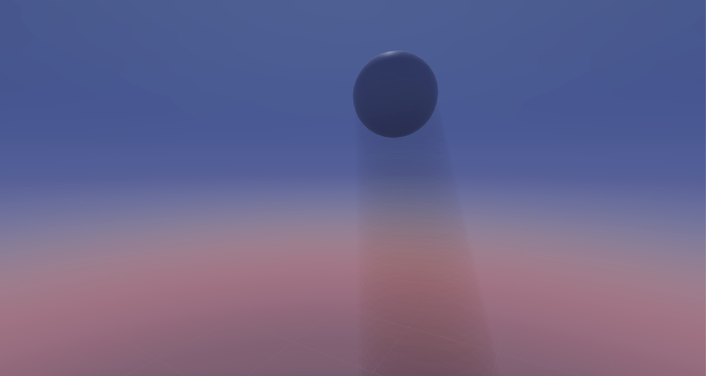
Integration
Thusfar, we’ve calculated atmospheric light scattering based off an atmosphere represented as a density function. This is a common approach for similar atmospheres in practically all games, but it’s precisely what makes the atmosphere arbitrary in most games. The density sampled by the atmosphere is defined by a constant function meaning it is static and cannot change no matter where you are in the world or what’s around you. It remains this way because many games cannot contain abstractions capable of parameterizing the atmosphere in a spatial, realistic way like what would be necessary to make it interactable.
That is except for our game! Handily enough, our map describing the terrain around the viewer contains a definition for density, which happens to be what the atmospheric integral is conceptually sampling. This density is used to define the liquid and solid surface, but in open-air its value is consistently below the IsoValue defining the ground meaning it serves no definable purpose except taking up space. Instead, we can visualize these values by evaluating them in our atmosphere repurposing them to describe all kinds of atmospheric effects. Moreover, this allows the game to become more unified; every system respects one true density and one true map.
Regrettably, this slows down calculations a lot. Firstly, optimizations assuming some sort of atmospheric pattern with the camera position and angle(as discussed previously) are impossible because the atmosphere becomes fundamentally unpredictable. Secondly, sampling from the map requires reading from regions of memory, which is much more inefficient than a function because calculations can no longer only be sourced from registers and caches–the GPU core must spend significant time traveling to shared memory. These problems necessitate significant optimizations which will be discussed in a future article.
Density
Map entries are confined to grid corners which are located at exact rigid positions in space. However, our atmospheric scatter integral is evaluated at regular intervals on an arbitrary camera ray, meaning we ideally want to evaluate the density at an arbitrary 3D point. We can do this by trilinearly interpolating the eight closest grid entries by the relative position of the 3D point we’re sampling–basically blending the densities in the voxel our point is in. Doing this means we obtain a continuous density that can be sampled for any arbitrary position.
The tradeoff is that we must sample 8 entries instead of one, greatly reducing efficiency. Ideally there should be a way to evaluate each entry only once along a ray by marching along the map down the ray, evaluating voxels one by one, and considering each density by the inverse distance from the entry to the line, but this offers less freedom for resolution and mathematically still needs a lot of work.
Recalling a previous article, we’ll remember that a single chunk may not completely contain the information necessary to describe the space bounded by it. Consequently, a point near a border of a chunk will find the corner entries describing its density lay in two seperate chunks, which might not even be the same resolution. Resolving this properly is almost always not justifiable just by how many more instructions it would necessitate. Hence, some error is accepted for samples near the border of a chunk.
Properties
Currently, the atmosphere is parametrized through density, but this only can control the thickness of the atmosphere. For a more varied/interesting atmosphere, it would be nice to also parametrize what type of light is scattered. For that, our map conveniently groups entries by a “material” which dictates the apperance for geometry originating from the entry. Realistically, each ‘material’ should describe a different type of particle which could reflect light differently depending on different atmospheric properties(e.g. scattering coefficient).
Defining unique scattering coefficients for every material(three for every primary color), requires the scattering coefficient to be factored within the integral(because it changes per every material). Likewise it would also be nice to customly define the extinction coefficient for different materials which must therefore also be evaluated similarly. With these defined, complex atmospheric structures like clouds, storms, tornadoes, mist or colored smoke can be replicated by simply manipulating the material of nearby entries.
It’s important to note that if these properties are to be blended in the same way as density(i.e. through a trilinear intepolation), the actual properties must be blended rather than the materials. The materials are discrete indexes pointing to properties in other LUTs and should not be mixed. If one were to blend the material, they would recieve a fractional lookup index which makes no sense. Conversely, this means the more properties a material has, the longer it will take to blend as each of the properties will need to be sampled 8 times and then blended individually, so care should be taken to reduce the amount of them.
Code Source
Basic Unoptimized Function-Based Atmosphere Shader
1 | Shader "Hidden/Fog" |
HLSL Sample Optical Map Data
1 | #include "Assets/Resources/Utility/GetIndex.hlsl" |