Atmospheric Acceleration

Atmosphere

 2024/09/22 

Overview

An elegant solution is commonly a simple system that can solve a number of problems. For instance, one may view the cosmos as elegant due to how a few simple laws governing elementary particles can create such complex experiences. Whether these laws are actually ‘simple’ or ‘few’, physicists may disagree, but even so the point stands that we often want to imagine it this way because it somehow feels better that the universe is minimally arbitrary so that all our experience can be derived from an innevitable causality.

This idea applies to any system whereby many problems individually solvable in painstaking case-by-case patches can be unified in a singular solution. Particularly, there are many aspects beneficial, or even indispensible, to modern open-world exploration games that often are resolved through single-purpose solutions. However, aside from being less ‘elegant’ these approaches are tangibly less scalable than a unified generic solutions which may be applicable to situations outside the single-case they were designed to resolve.

But there’s a reason single-purpose solutions exist. Even if physics were destructable to a basic set of particles and instructions, there is no computing system capable of simulating all the interactions necessary to support any meaningful simulation on a macroscopic scale. Single-purpose solutions simplify complex emergent behaviors meaning that they are often much more efficient at their specific task. Simultaneously, unified solutions may need significant optimizations to achieve a similar performance.

Background

Previously, a general algorithm for simulating atmospheric scattering was outlined in its primitive form. As the primary focus then was to create a generic function defining this effect, little care was given for its efficiency and, consequently, it suffers heavily from poor performance. Our scatter-function is meant to be process in realtime as it has to accurately simulate atmospheric scattering for a dynamic camera orientation. This implies that the function must be recalculated for every frame to not limit the camera’s refresh rate. But, the current model is far from being this fast on commercial devices and takes many seconds to calculate a single frame.

To illustrate the severity of this issue, we can consider the total amount of calculations our model will have to complete. Our algorithm currently sources its information from a central map stored in shared memory; this is far more inefficent than a simple arithmetic caclulation which can be contained entirely a core’s registers. To sample the density for a single point within the atmosphere, it performs a trilinear interpolation of the nearest 8 samples, requiring us to visit 8 memory locations.

Our algorithm must then approximate two nested integrals calculating out-scattering along two rays; the benchmark standard here for an acceptable approximation is usually 5 segments, though I will use 8 because it’s a power of 2. Then our algorithm must approximate the outer in-scatter integral by performing these operations for a new range of segments, these ones requiring much more detail–around 64 segments for a decent quality. Even then, we’ve only calculated the information for a single pixel on the screen, meaning we’ll have to repeat this process millions(2mil in standard 1080p) of times for standard commercial screens.

Counting it all up, this equates to roughly 8 * (8 * 2) * 64 * 2,073,600 or roughly 18 billion memory accesses every frame. Nowadays, a single DRAM access can take as little as 20-35ns, which means our program, at absolute minimum (remember we also have to locate the memory address, identify its properties, process multiple wavelengths, etc), can take about 340 seconds to complete! Of course, we haven’t factored in the possibility of parallel computation, but it’s still far from the 20ms benchmark of perceptible latency (also the GPU probably has other things to do in the frame).

It’s obvious to see that our algorithm won’t be fast. In fact, one of the earliest challenges in graphics programming was reconciling a similar model to evaluate in realtime. Luckily, this also means there’s a lot of work on the subject which we can reference to accelerate it. Consequently, like many problems in CS, optimization will be a process of picking and choosing algorithms and strategies to fit our specific implementation.

Specifications

To identify which optimizations we can apply without sacrificing too much visual quality, we should keep in mind the requirements of our model. Many algorithms(like that in our previous article), seek to simplify the calculation by locating identities between different rays so that they only need to be calculated once. This relies on the principle of the atmosphere being predictable: represented by a predictable function. With our model, however, since density is based upon an algorithm optimized to be random, and in fact is random once the user modifies it, such simplifications are capable of massive oversight, if not straight out impossible.

As our model can’t simplify the integrals constituting the bulk of our calculations, we have to search for other ways of reducing the amount of calculations while preserving a respectable quality. As a matter of fact, the essential principle of this article will be adhering to this fine line to increase performance by reducing quality in places where the user least sees the difference.

Solution

Down Sampling

If we take a look at the factors constituting our previous estimation for the total amount of calculations, we find that the most significant contributor is in repeating our calculations across every pixel on the screen. Since each pixel signifies a unique ray traversing the atmosphere, there are no obvious identities consistent enough to allow simplifications using data from other pixels. The only way to maintain the verity of a full-screen render is to evaluate our model across all its pixels.

On the other hand, the final result of atmospheric scattering between two adjacent pixels are usually very similar, so perhaps our proposed 2mil+ pixels is a bit excessive. Rather counterinuitively, our current algorithm could run faster on lower-end devices purely because a smaller screen means drastically less computations. To overcome this, we could virtually simulate a smaller screen and then enlarge it to our modern 1080p screen; in other words we can ‘downsample’ the calculation.

Achieving a lower sample screen than that of our maximum resolution should be relatively straightforward. If the pixel position is represented through a 2D UV Map (range 0->1) which can be transformed through a series of matricies to identify the camera ray along which our integral is calculated, we can simply traverse the UV map with a different resolution to obtain the ray information for a smaller screen. The problem is enlarging our small screen onto our high-resolution real screen.

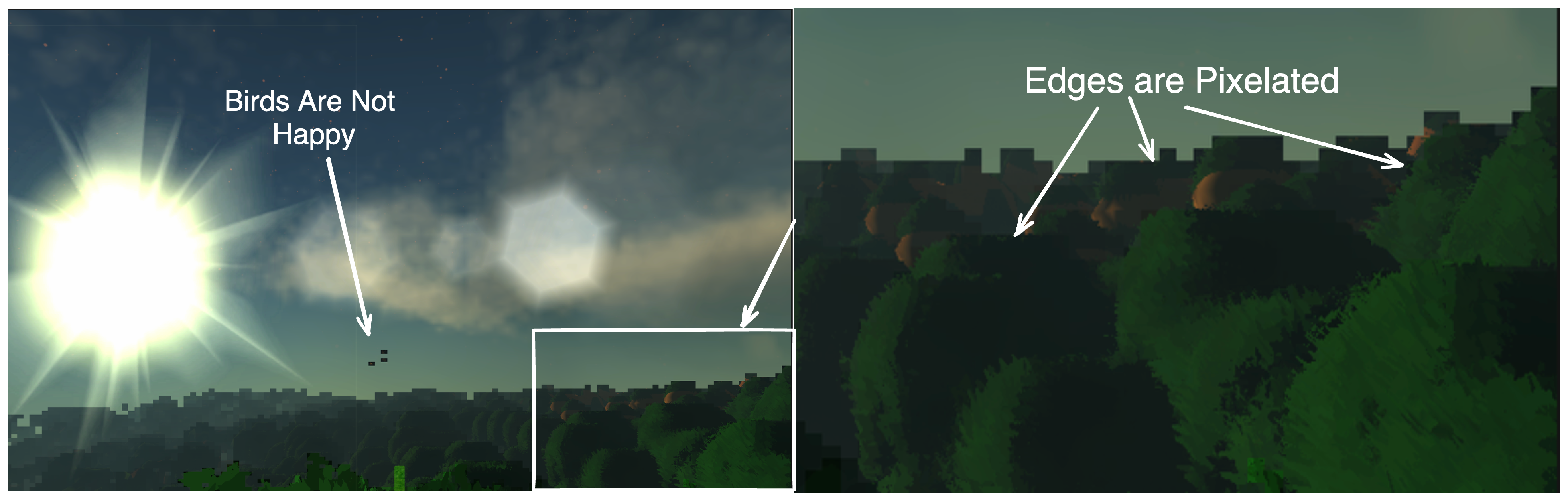
If we again represent the pixel position of a pixel on our high-resolution screen as a UV coordinate, we can scale it by the size of our small screen to obtain the closest samples which are located at the four nearest integer coordinates. If we simply take the values cached at the closest sample, we’ll find that our final screen becomes extremely blocky.

float2 pixelUV;
float2 SampleCoord = pixelUV * SampleScreenSize.xy;
int SampleIndex = LinearEncode ((int)round(SampleCoord), SampleScreenSize.xy);
return OpticalData[SampleIndex];

Essentially, it’s as if we just displayed our smaller sample screen as the result. Consequently, the edges of the smaller screen’s pixels become very obvious culminating in a very pixelated atmosphere. To obtain a smoother result, we can blur the result when enlarging from our smaller sampler using an old friend, bilinear interpolation. Basically, we can scale the contribution to a full-resolution pixel from the nearest four samples by the distance from each sample to the pixel. Doing so produces a continuous blend function across pixels ensuring a smooth result.

The benefit of blending our result is that it allows us to reduce the sampling size drastically with little visual drawback. Obviously there’s a limit to this and the quality difference does eventually become noticable, but considering simply halving the texture size increases throughput by a factor of 8, any reduction in size still drastically improves performance.

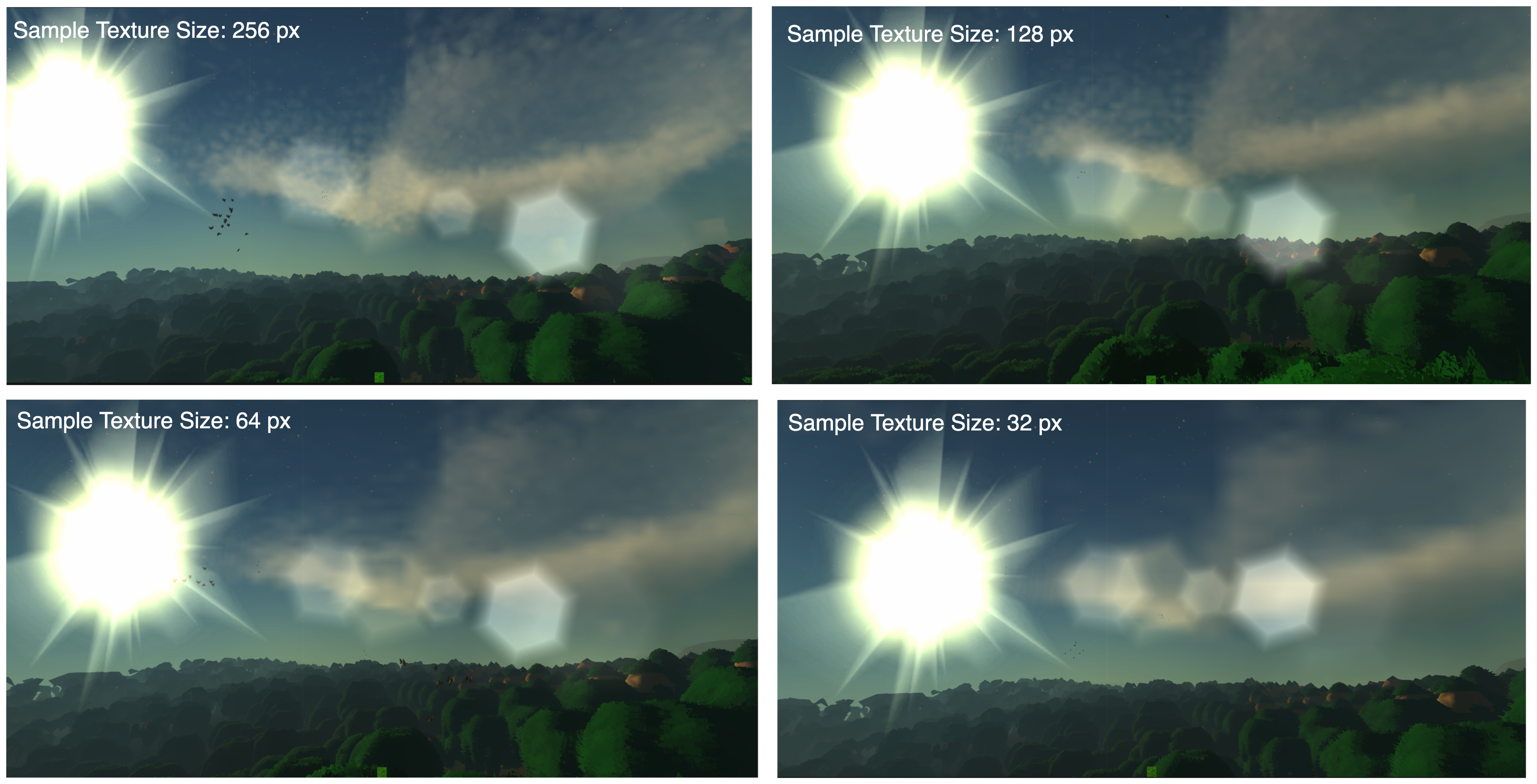
While the background sky gradient suffers minimally from the reduction in quality, we can see that excessive simplification can very obviously detriment spatially locked features like clouds. However, the difference in quality with progressively increasing sample size diminishes exponentially; above 256px the difference in visual quality is extremely minimal. Nevertheless even with a relatively big sample size of 256px, we are computing 32 times less computations than on a standard 1080p screen–such a difference that we are approaching realtime rendering.

Intermidiate Caching

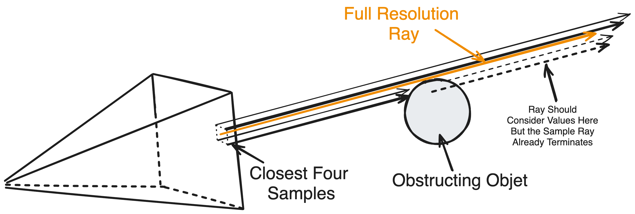
There’s a subtle yet pivotal problem with this simplification. Our model for atmospheric scattering calculates the contribution of light along a ray until the ray is obstructed. Light should not be able to reach us if it’s behind a surface so it makes sense to only evaluate the scattering integral up to the distance to the obstructing surface, or depth, of the pixel. If we apply the same logic to our downsampled pixels, and then upscale the result to our larger screen where each pixel ascertains its information from the closest low-resolution samples, a fatal oversight may occur where the depth of our full-resolution pixel is significantly different than that of the samples.

The reason this is so noticeable is because for abrupt changes in depth, such as across the edge of an object, a few samples may be obstructed early on by a surface while the rest extend to the edge of the atmosphere. If we were to suppose a ‘correct’ output given by evaluating the scatter equation at our exact full-resolution pixel location, that ray may extend to the edge of the atmosphere behind the end of several samples we’re blending from. Consequently, a significant portion of the ray can deviate from what’s expected as ideally it should reference a sample which extended as far as itself. This is true for any ray referencing the same sample with a depth significantly different than it–creating a pixelated edge along the border of objects.

For a second, if we forgo the sample’s depth and simply extend its ray to the edge of the atmosphere, regardless whether it’s occluded or not, and then blend the result for our high-resolution pixel, we can prove with absolute certainty that more light is in-scattered in this new result than our ideal ray (because this ray always extends to the end of the atmosphere). If we just scale down this result by the relative depth of our pixel, we run the risk of misrepresenting unproportionally dense regions along the ray which may reflect more or less light. Instead, if we split the ray into several regions and store the contribution of these sections individually, a full-resolution pixel can selectively choose which sections to blend depending on its specific depth.

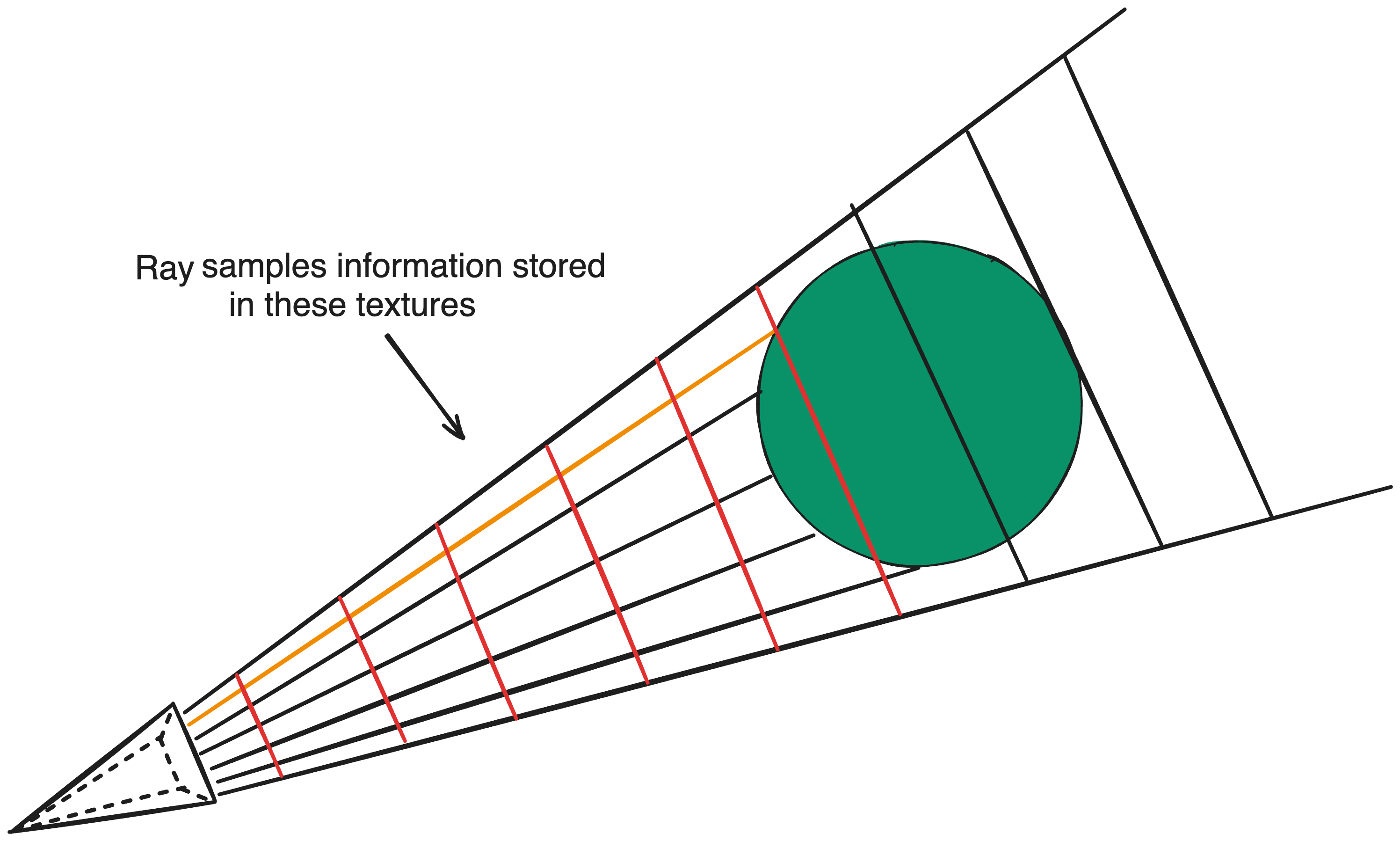
Considering a single pixel, the contribution at different depths can be envisioned as an array of values. But for a screen texture with a 2D grid of pixels, the aggregate contribution of each pixel at different depths can be represented by a 3D texture, where the texture index indicates the specific depth of all pixels writing to the texture. For maximum efficiency, one should encode this depth as the minor axis int index = x * size.yz + y * size.z + depth to optimize cache efficiency for the thread responsible for summing the segments.

Approximating Density

As we want our atmospheric algorithm to be an accurate reflection of our in-game information, there is an abnormal requirement for accuracy. While our proposed 64 segments is perhaps excessive for many function-based implementations, we should ideally want as many segments as map entries along our ray so that we don’t miss anything. This is because if an extraordinarily prominent feature(maybe a cloud or smoke particle) were only sometimes visible coinciding randomly with the camera orientation, it could induce a rather inconsistent and displeasing experience. For moderately large open terrains, hundreds to thousands of entries may exist along a ray meaning 64 segments is grossly inadequate.

If we simply increase the number of segments, our performance quickly falls off as each segment also must evaluate two other nested integrals for each new segment. If we rephrase our approximation as a riemann sum, such an approach would imply increasing the amount of terms in the summation. Instead, we can improve our accuracy by obtaining a better approximation for each segment.

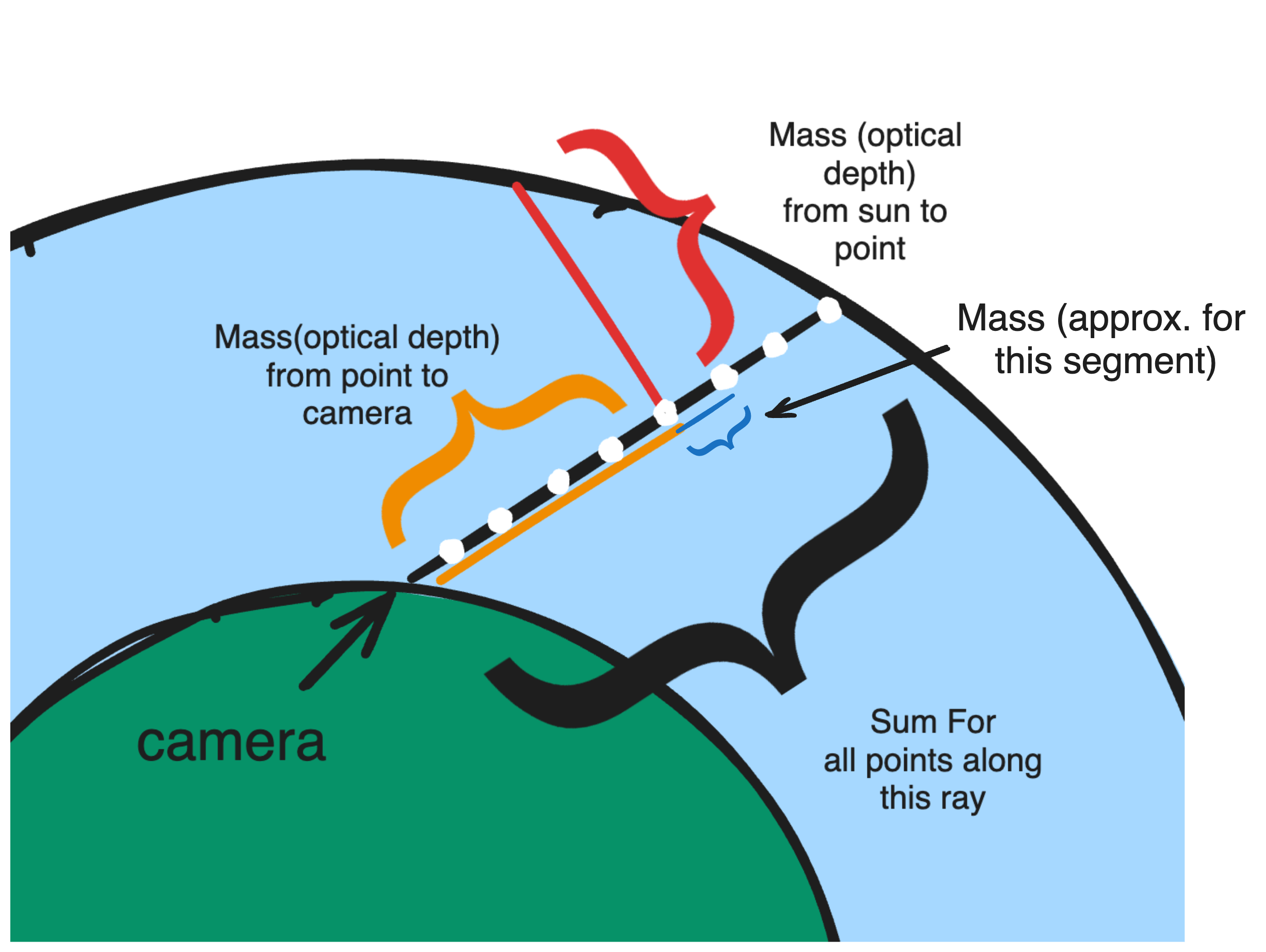
Referring back to the inscattering equation, the light from the sun is diminished by the outscattering integrals and multiplied by the specific density of the point. For an approximating segment, we ideally want to find the mass across the segment, which we can obtain by sampling it at any position in the beginning, middle, or end of the ray and scaling it by the length of the ray. But a more accurate approach is to approximate this mass as well through a seperate integral this time along the exact segment we’re approximating.

Computationally, since we aren’t approximating the other rays along the segment, this new calculation doesn’t compound but is rather just a third nested integral meaning the total amount of calculation for our equation is 8 * (8 * 3) * 64 as a pose to 8 * (8 * 2) * 8 * 64. Moreover, the improvement in visual detail is incredible, since our algorithm now is capable of evaluating the contribution of 512 seperate samples along the ray.

Binary Sum Tree

Reflecting on our changes, we can see how much of an improvement we’ve made; using a sample resolution of 128px, we can find that we’ve reduced our complexity to 8 * (8 * 3) * 64 * 128 * 128 = 201,326,592 calculations–which is almost 1% the amount of our original model. Unfortunately, this estimation is incorrect because it fails to account for a critical bottleneck of our algorithm: upscaling the image. To upscale our sample, for every full-resolution pixel there is a need to sum the cached partial segments of its closest 4 neighbors up to the pixel’s depth. With a quick calculation we’ll find that this actually takes 1920 * 1080 * 64 * 4 = 530,841,600 calculations for 1080p.

Since our information is subdivided between individual segments, acquiring the combined information for a pixel could require us to traverse a significant number of segments. If one tries to minimize the amount of partial segments, then we end up maximizing the depth error a pixel experiences as it cannot cull light around the end of its ray as finely as before. But as it is, the current method of summation introduces a lot of redundancy as many pixels sum the same partial segments as other pixels referencing the same sample. Fundamentally, if a pixel’s depth is farther than its neighbor, then the neighbor must’ve already calculated a portion of the partial sum for a sample that the current pixel is recreating.

Alternatively, we can expedite this process by precomputing portions of the summation in a binary sum tree. Basically, we can precompute the partial sum for every segment with its adjacent sibling segment to construct a tree where the root contains the entire summation along the entire ray. Then, to determine the summation for a specific depth, we can traverse the tree until the leaf segment closest to the depth. One can prove that with such an approach, our pixel will only traverse at most log₂n nodes, where n is 64 in our case.

Given that the amount of original segments whose sums we’re precomputing is N, the total amount of nodes in a binary tree is exactly 2*N supposing N is a perfect power of 2. Thus, representing a tree for each sample only doubles our base memory requirement, though it does get more difficult to visualize. Optimally, the minor axis should identify the index within a tree to benefit the cache efficiency for the thread searching through the tree; if one were to represent this as a 3D texture, this would be equivalent to storing a tree as a single row in a texture, and the pixel position encoded by the row and texture index.

The issue is with constructing this tree. Supposing that we start with one logical thread at each leaf node: so 64 threads are responsible for constructing every tree. Allowing all these threads to construct the same tree simultaneously, we get an intelligible mess because there is no guarantee that a segment has written its optical information by the time its sibling tries to take their sum. To construct the tree this way, it’s necessary we have a lock to determine when all segments have finished to allow the final thread to construct the tree. But this is highly inefficient. More processors does mean more synchronization issues but it simultaneously means more processing power. Making one thread construct our tree while all other threads wait for it is an extremely inefficient use of our resources; in principle, the best strategy would be to divide the task between each processor which constructs an equal portion of the tree.

To do this, we’ll have to use some clever strategies. First, let’s assume that the task of precomputing the partial sum for any node spanning two child segments will be completed by a thread that processed one of the child segments. For this thread to compute the sum, the information for its sibling node must already exist otherwise the task is impossible. If its sibling’s information exists, then our current thread should be responsible for writing its parent. Otherwise, we can assume that the sibling thread has not reached our node yet so our thread can terminate knowing that its sibling thread will have sufficient information to compute the summation when it reaches the node. In this way, each thread constructs a seperate portion of the tree depending on the order they are processed, and only the slowest thread constructs the root node. Furthermore, for any individual processor, the maximum number of nodes that it can be responsible for constructing is log₂N.

Now what we need is a synchronized way of indicating that a node is written to. Luckily, most standard languages have a set of atomic functions we can take advantage of. Particularly, we can use InterlockedXor to create a lock system to facilitate our task. Physically, when we xor two numbers we are telling the ALU to flip all the bits in the first number whose bits are 1 in the second. For example, in 13 ^ 6 we flip the bits ‘10’ in 1101 indicated by the two ‘1’s in 6(0110) to get 1011(or 11). By this logic, to flip a single bit stored in a sequence, we can utilize xor and use our operand to indicate which bit to flip.

1
2
3

bool FlipBit(int flagIndex){
    return (InterlockedXor(ref FlagStream, 1 << flagIndex) >> flagIndex) & 0x1;
}

In many languages, atomic operations return the value they replaced. Therefore, by the nature of xor flipping the bit, in the case where two threads InterlockedXor the same memory location with the same flagIndex, we can guarantee that they will be returned different results. Specifically, one will be returned the original value and the other, one with the opposite state of the specific flagIndex. We can use this to our advantage if we assume that the flag-bit was originally 0; if a thread is returned 1 by InterlockedXor on the location, another thread must have already flipped the bit before it. By extension, we can assume that this other thread must also have completed all tasks before the instruction as well.

With these facts, we can prove several things. Firstly, if two sibling threads contain instructions to first write their information to their node and then performed InterlockedXor on the same memory location, if a thread is returned 1 by the Xor then its sibling thread must have already written its information to its node. Secondly, since we can show that one of the two threads must recieve 1, if we designate the thread that recieves one as responsible for constructing the parent, all parents will innevitably be created by a thread.

The beauty of this algorithm is that flipping a bit twice will return it to the same state it was originally. So by the end of our algorithm the flag stream is returned to the same state it originated in. That means if our algorithm originated in its initialized state, it doesn’t require active zeroing to return it to that state after our algorithm modifies it as it will innevitably be returned to the same state anyways.

Finally to calculate the summation for any specific depth we can traverse down our tree and add our leftmost child if it’s encapsulated by our ray. A top-down approach like this is very obvious, but building a bottom-up traversal can often save small calculations which add up over time. To do this, if we obtain the depth divided by the length of a leaf segment, or the amount of segments we originally needed to sum, we can devise a traversal algorithm that starts at the bottom end-leaf segment of the tree, and moves up and across the tree summing all segments fully encompassed by the ray.

OpticalInfo SampleScatterTree(float rayLength, float sampleDist, uint2 tCoord){
    uint depth = ceil(rayLength / MaxNumDepthTextures) + MaxNumDepthTextures;

    //The leaf segment has to be handled differently because of the remainder depth
    OpticalInfo info = OpticalInfo[GetTextureIndex(tCoord, depth)] * fmod(rayLength, sampleDist);
    depth--;

    while(depth > 0){ //Operator precedence is == then & 
        if((depth & 0x1) == 0) {
            info += OpticalInfo[GetTextureIndex(tCoord, depth)];
            depth--;
        };
        depth >>= 1; //Go to its parent
    }
    return info;
}

With the algorithm above, it’s very clear how the algorithm provides a logarithmic lookup time. Furthermore there’s less variables tracking temporary traversal data that’s relevant in other top-down approaches.

Other Strategies

Depth Binding

Admittedly, this isn’t the only way to expedite the process of upscaling. If you’ll remember, the whole point of intermediate caching is because the specific ray depth of our full-screen pixel may vary largely from the sample’s depth. This is only really prominent near edges of objects so for most of the screen the pixel’s depth and the sample’s is roughly the same. This implies that for most pixels, the whole process of intermidiate caching and partial summation is redundant and only serves to slow the system down.

Realistically, if all pixels that rely on a certain sample are above a specific depth, there’s no need to intermediately cache segments within that range as no pixel will need to differentiate between them. It would be better if we just coalesced these segments into a single segment of a length equivalent to that minimum depth, that way when upscaling we don’t need to needlessly recalculate it. To find this minimum depth, we have two options.

We can process each full-resolution pixel using a seperate logical thread and InterlockedMin its depth with that of the nearest 4 samples.
We can process each sample position using a seperate logical thread, and evaluate the depths of every full-resolution pixel that can reach it to find the minimum.

The second strategy is preferred because it’s of the same thread distribution strategy as our sampling step, meaning there’s no need for a second synchronization step between them. Additionally, we would need to max-out the sample depth before computing the minimum in the first strategy which is not a concern in the second as each thread controls its own exclusive sample. By the same process we can determine the maximum depth of any pixel referencing a sample. This can save us processing power as calculating partial segments past the maximum depth is pointless and the extra segments can be repurposed to increase the quality of our approximation.

There is a notable overhead with this strategy. As each sample measures the depth of all full resolution pixels referencing it, and a full resolution pixel is capable of referencing 4 samples, collectively we’re remeasuring the depth of every pixel 4 times, or computationally sampling a texture twice(in each dimension) the size of our screen. Considering how some depth textures may be cascaded or of a different resolution than the screen, sampling a single pixel often involves sampling 4 seperate memory locations and taking a bilinear blend. This can accumulate into a significant drawback for those considering this strategy.

Morton Encoding

A final improvement to increase speed is to encode either the terrain map or the sample LUT using morton encoding, or bit interleaving. For samples along a ray, traditional linear encoding isn’t very efficient as traversing against the major axis will require the cache to jump across large regions of memory. By using morton encoding, cache data is located more genuine to its spatial orientation, meaning that a thread approximating samples along a ray could experience far less cache misses.

Of course this is all just in theory. In reality, cache efficiency is a concept shrouded behind many many layers of abstraction that could completely undermine this idea in extremely complicated and obscure ways. While on paper morton encoding should significantly increase performance there isn’t much of a difference in my experience. Generally, however, if optimizing an algorithm’s cache coherence is a huge concern for improving performance, it’s already a sign that the algorithm is approaching its efficiency limit.

Code Source

Optimized HLSL Sample Intermediate Caching and BST Construction

#pragma kernel Bake
#include "Packages/com.unity.render-pipelines.universal/ShaderLibrary/Core.hlsl"
#include "Packages/com.unity.render-pipelines.universal/ShaderLibrary/Lighting.hlsl"

#include "Assets/Resources/Utility/GetIndex.hlsl"
#include "Assets/Resources/MapData/WSDensitySampler.hlsl"

struct ScatterData{
    float3 inScatteredLight;
    float3 extinction;
};

RWStructuredBuffer<ScatterData> mapData;
RWStructuredBuffer<uint> treeLocks;
StructuredBuffer<float3> rayInfo;
uint screenHeight;
uint screenWidth;

float3 _LightDirection; //Global Variable

float _AtmosphereRadius;
uint _NumInScatterPoints;
uint _NumOpticalDepthPoints;
float _IsoLevel;

float2 raySphere(float3 s0, float sr, float3 r0, float3 rd) {
    float a = dot(rd, rd);
    float3 s0_r0 = r0 - s0;
    float b = 2.0 * dot(rd, s0_r0);
    float c = dot(s0_r0, s0_r0) - (sr * sr);
	float disc = b * b - 4.0 * a* c;
                    
    if (disc < 0.0) {
        return float2(-1.0, -1.0);
    }else{
        float t1 = max((-b - sqrt(disc)) / (2.0 * a), 0);
        float t2 = max((-b + sqrt(disc)) / (2.0 * a), 0);
        return float2(t1, t2-t1);
	}
}

float calculateOcclusionFactor(float3 rayOrigin, float3 rayDir, float rayLength){
    half cascadeIndex = ComputeCascadeIndex(rayOrigin);
    float stepSize = pow(2, cascadeIndex);
    int NumShadowPoints = max(1, rayLength / stepSize);

    float3 shadowPoint = rayOrigin;
    float transmittanceCount = 0;

    for(int i = 0; i < NumShadowPoints; i++){
        transmittanceCount += MainLightRealtimeShadow(TransformWorldToShadowCoord(shadowPoint));
        shadowPoint += rayDir * stepSize;
    }
    return (transmittanceCount / NumShadowPoints);
}

OpticalInfo CumulativeMapInfo(float3 rayOrigin, float3 rayDir, float rayLength){
    float3 densitySamplePoint = rayOrigin; 
    float stepSize = rayLength / (_NumOpticalDepthPoints - 1);
    OpticalInfo info = (OpticalInfo)0;
    for(uint i = 0; i < _NumOpticalDepthPoints; i++){
        OpticalInfo sampleData = SampleMapData(densitySamplePoint);

        info.opticalDensity += sampleData.opticalDensity / (_IsoLevel * 255.0f);
        info.scatterCoeffs += sampleData.scatterCoeffs;
        info.extinctionCoeff += sampleData.extinctionCoeff;

        densitySamplePoint += rayDir * stepSize;
    }
    info.opticalDensity /= _NumOpticalDepthPoints;
    info.scatterCoeffs /= _NumOpticalDepthPoints;
    info.extinctionCoeff /= _NumOpticalDepthPoints;
    info.scatterCoeffs *= calculateOcclusionFactor(rayOrigin, rayDir, rayLength);
    
    return info;
}

float3 opticalDepth(float3 rayOrigin, float3 rayDir, float rayLength){
    float3 densitySamplePoint = rayOrigin;
    float stepSize = rayLength / (_NumOpticalDepthPoints - 1);
    float3 opticalDepth = 0;

    for(uint i = 0; i < _NumOpticalDepthPoints; i++){
        OpticalDepth mapData = SampleOpticalDepth(densitySamplePoint);
        opticalDepth += mapData.scatterCoeffs * (mapData.opticalDensity / (_IsoLevel * 255.0f)) * stepSize;
        densitySamplePoint += rayDir * stepSize;
    }

    return opticalDepth;
}

void ConstructSampleTree(ScatterData cNode, uint pixelIndex, uint depth){
    depth += _NumInScatterPoints; uint parent = depth >> 1;
    uint numTreeLocks = ceil(_NumInScatterPoints / 32.0f);
    uint lockHandle = 0xFFFFFFFF;

    //Parallel Binary Index Tree Construction
    while(depth != 0){//>> 5 means / 32
        uint lockIndex = pixelIndex * numTreeLocks + (parent >> 5);
        uint texelIndex = pixelIndex * _NumInScatterPoints * 2 + depth;
        mapData[texelIndex] = cNode;

        InterlockedXor(treeLocks[lockIndex], 1 << (parent & 0x1F), lockHandle);
        if((lockHandle >> (parent & 0x1F)) & 0x1 == 0) return; 
        //If lock bit is 0, its sibling is second and has not completed yet
        //If lock bit is 1, its sibling is first, so we can safely access it 

        ScatterData sibling = mapData[texelIndex ^ 0x1];
        cNode.inScatteredLight += sibling.inScatteredLight;
        cNode.extinction += sibling.extinction;
        depth >>= 1; parent >>= 1;
    }
}


const static uint numThreads = 8;
[numthreads(numThreads,numThreads,numThreads)]
void Bake (uint3 id : SV_DispatchThreadID)
{
    uint viewX = id.x;
    uint viewY = id.y;
    uint depth = id.z;

    if(viewX >= screenWidth || viewY >= screenHeight || depth >= _NumInScatterPoints)
        return;
    
    uint pixelIndex = indexFromCoord2DManual(viewX, viewY, screenHeight);
    float3 direction = rayInfo[pixelIndex];

    float stepSize = _AtmosphereRadius / (_NumInScatterPoints - 1);
    float3 inScatterPoint = _WorldSpaceCameraPos + direction * stepSize * depth;
    float sunRayLength = raySphere(_WorldSpaceCameraPos, _AtmosphereRadius, inScatterPoint, _LightDirection).y; 

    ScatterData scatterData = (ScatterData)0;
    OpticalInfo opticalInfo = CumulativeMapInfo(inScatterPoint, direction, stepSize); 

    //Calculate Scatter Data
    float3 sunDepth = opticalDepth(inScatterPoint, _LightDirection, sunRayLength);
    float3 cameraDepth = opticalDepth(inScatterPoint, -direction, stepSize * depth); 
    float3 transmittance =  exp(-(sunDepth + cameraDepth)); // exp(-t(PPc, lambda)-t(PPa, lambda)) 
    scatterData.inScatteredLight = opticalInfo.scatterCoeffs * opticalInfo.opticalDensity * transmittance;
    scatterData.extinction = opticalInfo.extinctionCoeff * opticalInfo.opticalDensity;
   
    ConstructSampleTree(scatterData, pixelIndex, depth);
}

Optimized Upscale Shader. Final Render Result

Shader "Hidden/Fog"
{
    Properties
    {
        _MainTex ("Texture", 2D) = "white"
    }

    SubShader
    {
        Tags
        {
            "RenderType"="Opaque" "RenderPipeline" = "UniversalPipeline"
        }
        ZWrite Off
        
        HLSLINCLUDE
        #pragma vertex vert
        #pragma fragment frag
        #pragma multi_compile _ _MAIN_LIGHT_SHADOWS _MAIN_LIGHT_SHADOWS_CASCADE

        #include "Packages/com.unity.render-pipelines.universal/ShaderLibrary/Core.hlsl"
        #include "Packages/com.unity.render-pipelines.universal/ShaderLibrary/Lighting.hlsl"

        #include "Assets/Resources/MapData/WSDensitySampler.hlsl"
        #include "Assets/Resources/Atmosphere/TextureInterpHelper.hlsl"

        struct Attributes
        {
            float4 positionOS : POSITION;
            float2 uv : TEXCOORD0;
        };

        struct v2f
        {
            float4 positionHCS : SV_POSITION;
            float2 uv : TEXCOORD0;
            float3 viewVector : TEXCOORD1;
        };

        TEXTURE2D(_MainTex);
        SAMPLER(sampler_MainTex);
        TEXTURE2D(_CameraDepthTexture);
        SAMPLER(sampler_CameraDepthTexture);

        struct ScatterData{
            float3 inScatteredLight;
            float3 extinction;
        };

        StructuredBuffer<ScatterData> _OpticalInfo;
        float4 _MainTex_TexelSize;
        float _AtmosphereRadius;
    
        int _NumInScatterPoints;


        v2f vert(Attributes IN)
        {
            v2f OUT;
            OUT.positionHCS = TransformObjectToHClip(IN.positionOS.xyz);
            OUT.uv = IN.uv;

            //Z is forward
            float3 viewVector = mul(unity_CameraInvProjection, float4(IN.uv.xy * 2 - 1, 0, -1)).xyz;
			OUT.viewVector = mul(unity_CameraToWorld, float4(viewVector, 0)).xyz;

            return OUT;
        }
        ENDHLSL

        Pass
        {
            Name "Fog"

            HLSLPROGRAM
            float2 raySphere(float3 s0, float sr, float3 r0, float3 rd) {
                float a = dot(rd, rd);
                float3 s0_r0 = r0 - s0;
                float b = 2.0 * dot(rd, s0_r0);
                float c = dot(s0_r0, s0_r0) - (sr * sr);
	            float disc = b * b - 4.0 * a* c;
                    
                if (disc < 0.0) {
                    return float2(-1.0, -1.0);
                }else{
                    float t1 = max((-b - sqrt(disc)) / (2.0 * a), 0);
                    float t2 = max((-b + sqrt(disc)) / (2.0 * a), 0);
                    return float2(t1, t2-t1);
	            }
            }

            ScatterData SampleScatterTree(float rayLength, float sampleDist, uint2 tCoord){
                uint depth = clamp(floor(rayLength / sampleDist) + 1, 1, _NumInScatterPoints - 1) 
                              + _NumInScatterPoints;
                //Get precision for last point
                ScatterData scatterData =  _OpticalInfo[GetTextureIndex(tCoord, depth)];
                scatterData.inScatteredLight *= fmod(rayLength, sampleDist);
                scatterData.extinction *= fmod(rayLength, sampleDist);
                depth--; 

                while(depth > 0){ //Operator precedence is == then & 
                    if((depth & 0x1) == 0) {
                        ScatterData cScatter = _OpticalInfo[GetTextureIndex(tCoord, depth)];
                        scatterData.inScatteredLight += cScatter.inScatteredLight * sampleDist; //256
                        scatterData.extinction += cScatter.extinction * sampleDist; //256 
                        depth--;
                    };
                    depth >>= 1;
                }
                return scatterData;
            }

            ScatterData CalculateScatterData(float rayLength, float sampleDist, Influences2D blend){
                ScatterData scatterData = (ScatterData)0;
                [unroll]for(uint i = 0; i < 4; i++){
                    if(blend.corner[i] == 0) continue;
                    ScatterData cScatter = SampleScatterTree(rayLength, sampleDist, blend.origin + uint2(i & 1u, (i >> 1) & 1u));
                    scatterData.inScatteredLight += cScatter.inScatteredLight * blend.corner[i]; //4
                    scatterData.extinction += cScatter.extinction * blend.corner[i]; //4
                }
                return scatterData;
            }

            half4 frag(v2f IN) : SV_TARGET
            {
                half4 originalColor = SAMPLE_TEXTURE2D(_MainTex, sampler_MainTex, IN.uv);
                float screenDepth = SAMPLE_DEPTH_TEXTURE(_CameraDepthTexture, sampler_CameraDepthTexture, IN.uv);
                float linearDepth = LinearEyeDepth(screenDepth, _ZBufferParams) * length(IN.viewVector);
                float3 emissionColor = _MainLightColor.xyz;

                //Assume atmosphere originates at viewer
                float dstThroughAtmosphere = min(_AtmosphereRadius, linearDepth);
                Influences2D rayInfluences = GetLookupBlend(IN.uv);
                float sampleDist = _AtmosphereRadius / (_NumInScatterPoints - 1);

                if(dstThroughAtmosphere > 0){
                    ScatterData atmosphereData = CalculateScatterData(dstThroughAtmosphere, sampleDist, rayInfluences);
                    return half4(atmosphereData.inScatteredLight * emissionColor + originalColor.xyz * exp(-atmosphereData.extinction), 0);
                }
                return originalColor;
            }
            ENDHLSL
        }
    }
}

Author：Jonathan Liu

Link：https://blackmagic919.github.io/AboutMe/2024/09/22/Atmospheric-Acceleration/

Publish date：September 22nd 2024, 10:09:44 pm

Update date：January 17th 2025, 7:35:07 pm

Next Post

GeoShaders
Previous Post

Atmospheric Scattering

CATALOG

1. Overview
2. Background
3. Specifications
4. Solution
5. Code Source