
Overview
In the early era of digital gaming, there weren’t many splendid visual effects beyond what was functionally necessary. But as time went on, much larger portions of the public began to gain accessibility to increasingly powerful machines allowing developers to attempt to capture more and more intricate effects not previously thought feasible. As of today, many of these effects have amassed so much noteriety that their presence is almost expected of any high-end game. Notably, geometry shaders refer to a set of effects that have become commonplace in many new high-quality games.
A geometry shader(GeoShader), is commonly a name given to a shader stage that generates new geometry based on existing geometry from outside the render pipeline. As these new primitives are each generated from a base primitive, they usually inherit only information about their base primitive and thus are often used to elevate their base geometry rather than model a new shape. They are often used to enhance certain visual effects in a quick way and are traditionally used for complex visual features such as leaves, grass, hairs, smoothing, etc.
Background
Conventionally graphics systems render geometry through representing them as collections of triangles. This is because triangles are predictable–three vertices define a plane which has a unique normal, triangles can be partitioned into heiharchies to sort through when rendering, and they are an atomized unit which can be distributed across processors. At the same time, triangles are a versatile unit capable of representing practically any geometry given a large enough collection. That’s not to say triangles are the only way to render something; 2D models commonly simplify the need for variable depth geometry triangle-based rendering is built to solve, and other pipelines may be better in different situations (e.g. our Atmosphere pipeline).
Regardless, most applications requiring variable depth geometry take advantage of a general pipeline framework which, summarized, works by first determining all the triangles on the user’s screen, and then drawing the closest triangles to the pixels they overlap. Most developer-level shaders are by nature Surface Shaders which determine the color drawn to a pixel once the triangle it overlaps has been determined. As one could suspect, this stage takes in the triangle’s vertices and relative offset to them as its input and has no control over where the triangle it is responsible for is oriented.
The reason for this design choice is that a seperation of concern allows for expedited rendering as stages can facilitate parallelization of the pipeline–each task after a major stage can usually guarantee the previous stage’s task is complete. With this design, if the viewer wishes to draw geometry to a different location, they would’ve defined those polygons in their geometry buffers before it reaches the Surface Shader step. But sometimes, this is overly costly and a different solution is prefered.
Take grass for instance, in large outdoor terrains a Surface Shader can be used to overlay a grass texture where desirable, but this is lacking in many aspects. Of course, a more complicated surface shader could take advantage of the camera and light angle to emulate these effects, but ultimately the illusion is broken when viewed in front of another object because they cannot dictate the position of the geometry and where they’re rasterized to. On the other hand, if one were to declare these in the geometry buffer, it would require a lot of prior setup and maintenance on the CPU(considering the CPU generates the geometry).
To solve this, many modern pipelines allow for a stage(or sub-stage) for Geometry Shaders which generate new ephemeral primitives that only exist within the pipeline and is thus recreated everytime the pipeline executes(every frame). As such, they constitute a high cost/low maintenance & overhead solution for many simple effects that require on-demand geometry.
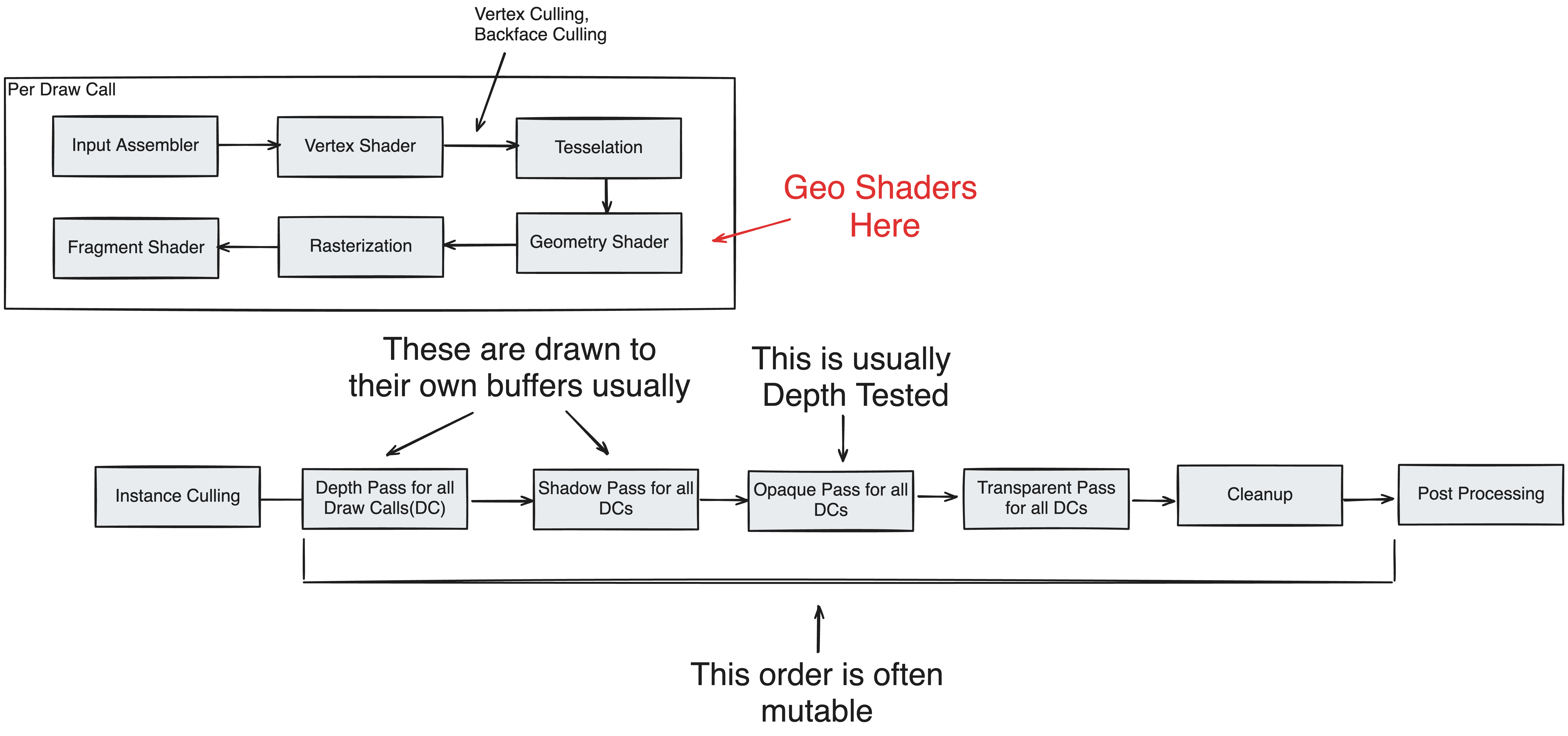
There are several disadvantages with conventional GeoShaders. Firstly, since they are an integrated part of the pipeline, they need to be regenerated every frame, or however often the camera is refreshed. This makes it a problem if a large amount of geometry is generated this way, as recreating and serializing the data every frame may cause significant load. Secondly, one might notice how vertex culling occurs before geometry shaders–this means that its geometry will always be processed by the rasterizer and pixel shader even if the primitive in question is backfacing, or not on the screen. Given a large amount of dispersed geometry, this can lead to significant unnecessary work contributing to latency. Since they’re designed to be lightweight, these design choices make sense but they do place an upper limit on how much geometry can be generated efficiently.
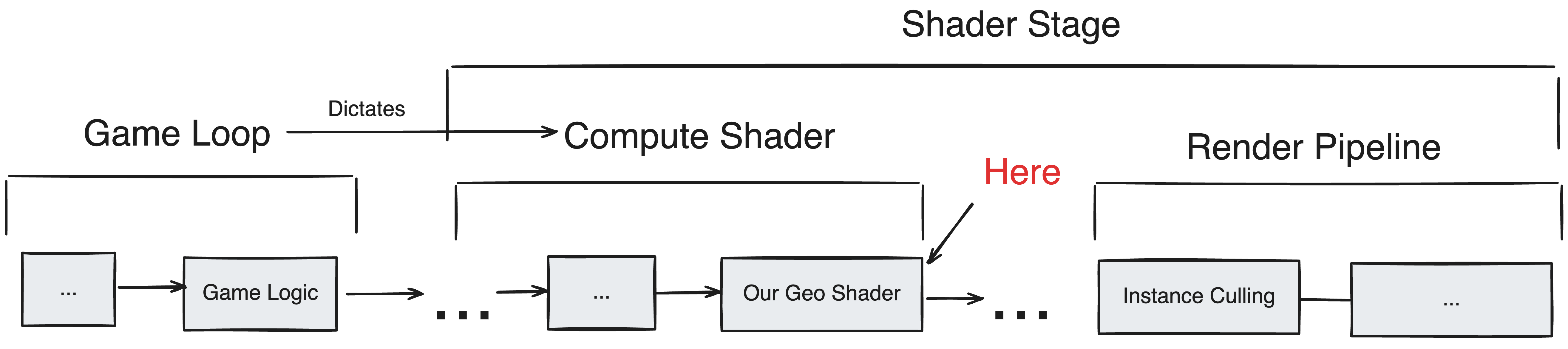
For these reasons, instead of a traditional GeoShader a custom system is applied which generates persistent geometry outside of the render pipeline. With regards to the pipeline this new geometry is treated identically to our authentic geometry, meaning it is capable of being culled and optimized. Despite these differences, this system will still be referred to as a “GeoShader” due to its resemblances to the design pattern of its integrated counterpart, being that it recieves a base primitive and returns new geometry. Primarily, the main benefit is in its lifespan–which is longer and requires less replacement.
It is important to remember this distinction, wherein “GeoShader” does not refer to the traditional render stage, but a onetime preprocessing compute shader step independent of the pipeline.
Batching
Problem
A common strategy of rendering objects with different apperances is to define a unique Shader/Material which includes its own logic on what to draw given some geometry. In doing so, each ‘logic group’, or shader, is its own draw call where all geometry with the shader is batched and drawn together. It is done this way because context switching is very slow on GPU architecture, so it is minimized in return for reduced parallelism. Maintaining a low amount of drawcalls(i.e. few unique shaders) is imperitive because fewer draw calls usually means less context switching and less synchronization.
The same is true of GeoShaders. Since each material would like to define its own generation logic, it is very expensive if each triangle searches for instructions on how to create geometry given its material. Not to mention, GPU cores usually preload a job’s instructions onto their cache before batch processing all tasks in its WorkerGroup(which will use the same instructions). If the instructions are too long, a core will be unable to load the instruction set in its entirety resulting in extreme slowdowns as each task in the WorkerGroup must reload the instructions as it progresses.
Instead, similar to draw calls, we need a method to batch all triangles with identical GeoShaders(same instructions) together. That way the GPU has time to preload their instructions on the core before batch processing them all at once. Moreover, this batching stage must be a GPU executable process so that it can be buffered into its execution without stalling our CPU (see Memory Heap).
Solution
To start, we can assume that we’re provided an unprocessed collection of geometry, or a collection of triangles where each triangle may describe its own GeoShading rules. To batch process all triangles with identical rules together, we need to know two key pieces of information for every batch: how many triangles are within the batch and how to determine which triangle to process for each thread in the batch. Once this information is known, it becomes very easy to formulate a cohesive batch where our available resources can be divided among the primitives such that each logical thread is able to find its own exclusive triangle to process.
Determining the amount of geometry can be accomplished provided we know how much geometry is in our collection. In this case, a shader can be used to divide threads for each triangle, whereby each thread would count their triangle through a shared counter utilizing an atomic increment(e.g. InterlockedAdd) if it is of the current batch. Then this process could be repeated for each batch leading to a total time complexity listed below.
1 | N = Number Of Triangles In Collection |
However if batches are mutually exclusive, and we know in advance the maximum amount of batches to be processed, what can be done instead is to allocate counters for all batches, and count all the batches in one swing. If each batch were assigned a unique ‘counter-index’, a thread could determine this index depending on its triangle’s GeoShader and increment a unique counter counting only geometry in its batch. That way all geometry in every batch can be counted in O(N/P).
Now comes the hard part. Once we’ve determined how many triangles are in each batch, we can request a corresponding amount of threads to process it whereby each thread must find a unique triangle within the batch. But as the base geometry is buried amongst an unsorted collection we have no way of finding this triangle. Ideally, if we could sort all triangles into their batches, this could be achieved by assigning an index to each thread, and finding the triangle within the sorted batch at that specific index; provided that indexes are assigned consecutively, this would ensure all triangles are processed given the batch count is correct.
Parallel sorting is very unorthodox for those familiar with traditional sorting algorithms primarily because it’s necessary to provide exclusive working areas for each processor. It’s a well-researched problem with many proposals, but generally, the time complexity approaches O(N log N / P) for a good implementation. Although this may already be satisfactory, there is a major simplification for us given that we know the number of unique batches in our collection. Since we know the size of each batch, we can assume that once sorted each batch will span a region within the array of that specific size. What’s more, if we assume that triangles are sorted by their batch’s counter index, what we find is that in the final sorted array, the index at which a batch begins is equivalent to the sum of all batch counters before it. Or phrased in another way, each batch can find its mutually exculsive start from the prefix sum of batch sizes up to itself.
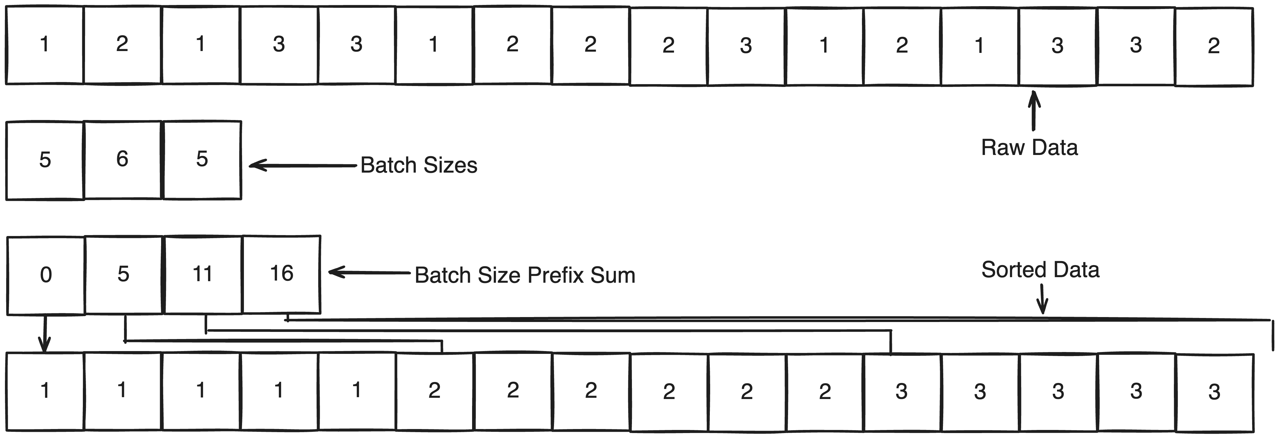
After ascertaining this prefix sum, each region within the sorted array can be thought of as its own seperate buffer whereby the remaining task of placing our data in the sorted array can be rephrased as appending each triangle into its batch’s buffer at a unique position in a way similar to how Unity handle’s Append Buffers. Underneath, Unity does this through a hidden counter and the clever use of an atomic increment, which returns the value it replaced as an atomic operation. As this atomic operation also increments the value upon reading, it ensures that no other thread can read the same value as by definition one must happen before another. Furthermore, the original prefix sum entries can be reused as the counters, indicating the next position a triangle of the batch will be placed in the sorted array.
In this way, our triangles can be sorted in O(N / P) whereby a thread may determine its triangle’s location through offsetting its thread index with the prefix start of its batch to find the entry within the sorted reference array containing the address of the triangle in the original collection.
Here’s a more effecient way to achieve the same effect. The returned index is retained when counting the batch sizes.
- Zero/Clear counters equivalent to the maximum amount of batches
- For all triangles in the geometry, determine what batch it belongs to(if it has a GeoShader) and atomic increment its respective counter. Retain the returned index as the triangle offset
- Construct a prefix sum synchronously from the counters for all batches
- For each triangle place it at the position that’s the sum of its GeoShader’s prefix sum entry and its specific triangle offset.
Unit Compression
Problem
While we could implement this straight away, there is an ethical concern we’re ignoring that is important for a robust system design. If our base geometry is populated by a large quantity GeoShaded primitives, a significant portion of memory will be spent on retaining the generated output. For a typical GeoShader, anywhere from 5 to 16 extra vertices may be generated for each base vertex–if we consider 1/2 of triangles are geoshaded(which isn’t a large number considering many grassy fields may be entirely geoshaded) we’ll find that GeoShaded Geometry may constitute more than 4 times as much vertices as our base geometry, as a conservative estimate.
In reality, Marching Cubes generates overlapping vertices, which when accounted for reduces vertex count by a factor of 4 exactly(ignoring edges). However, this doesn’t reduce the amount of triangles which are individually processed by GeoShaders meaning even if a GeoShader produced one triangle for every base triangle, it would innevitably create 4 times the vertices. One could attempt to reclaim these duplicate vertices, but as GeoShaders may vary this would be an arduous case by case undertaking.
This isn’t a concern for traditional GeoShaders, as GeoShaded geometry is not retained but discarded per draw call, the maximum amount is correspondingly limited by the maximum batch draw call size. Rather traditional GeoShader’s often limit the distance GeoShaders are applied primarily due to the rendering load. By the same reasoning, one could reduce our custom GeoShader’s memory load by limiting the distance at which they are applied. But even at the extreme, this could only be limited to the smallest LoD range at which chunks will regenerate, or the concept of retaining GeoShaded geometry breaks down.
Ultimately, utilizing 4-8x the of space our base geometry to store purely gratuitous visual effects not central to the simulation is questionable, so a form of unit compression is desirable.
Solution
Let’s start by defining the basic information each GeoShaded geometry might include. To be integrated within most standard renderpipelines it must specify its 3D position: usually 3 numbers describing its unique cartesian position in the world. Additionally, to determine lighting information for the primitive we must also specify the normal of our vertex–usually a 3D unit cartesian vector. Technically, as each plane has a ‘true normal’ specified as the cross product of two edges one could get away with not specifying it, but effects like smooth geometry would no longer be possible. Finally, we’ll add an extra number for GeoShader internal information, such as UVs if texture mapping is required. Sticking to 4-byte precision, that’s a total of (3 + 3 + 1) * 4 = 28 bytes per vertex.
Now, depending one one’s purpose for GeoShaders, it’s possible to design a compact representation where GeoShaded geometry is heavily reliant on its base information. For example, one could specify that GeoShaded geometry inherits its base triangle’s normals, completely eliminating 12 bytes, while its position is restricted to a limited offset from the base triangles center, feasibly reducing the 12 byte coordinate to 3 bytes. An extra 4 bytes would be needed to reference the index the triangle is based off of amounting to a potential total as low as 8 bytes. However, due to the amount of extra handles and pre-processing Surface Shaders need to account for to decode this information, it accumulates to a notably slower performance, not to mention severly limiting GeoShader potential.
If we limit the range of each coordinate of our normal cartesian vector to (-1, 1), we’re still capable of representing all normals of magnitude ≤ √3. As this is now a finite range, we can simply represent this as an integer, and downscale it by our desired precision. For example, if we resolved for 6 bit precision, we can divide our integer representation by 63.0(2^6 - 1) in IEEE754 for the ALU to return us our original number in floating-point.
But we can do better. If we specify that normals must be unit vectors(magnitude = 1), the spherical representation of our coordinates will necessarily be of the form (1, θ, Φ) (that is ρ = 1). This effectively eliminates one coordinate meaning we can represent all unit normals with two numbers. θ is traditionally of the range 0 < θ < 2π while Φ is bounded as 0 < Φ < π. If θ is represented with 8 bits and Φ with 6, we get the following formulas.
1 | float3 cartesian; //unpacked normal |
Of course many other normal packing strategies exist that may be just as efficient, but this one is sufficiently compact for our purposes. With it we can reduce our original 96 bits to just 14.
If our positions can assume any location in the world, it would be necessary to use a versatile representation such as floating-point to quantify them. But normally, geometry is grouped together into locally contained batches, whereby a common transformation(i.e. matrix operation) can be applied to transform the entire batch when rendering. What this means is that each triangle can specify its local transform to its batch rather than its ‘global position’ which usually gives a much tighter range.
In Arterra, each map entry is located at integer unit positions within its ‘local space’, or an arbitrary space where (0,0) is defined as the origin of the chunk. Since the maximum number of entries is declared as 64, all geometry within the chunk will have a local coordinate in the range (0, 64). Regrettably, our GeoShaders do not adhere to this as they’re are able to generate at any offset from a base geometry. But if we define a maximum offset, then we can declare an absolute range of values from (0 - offset, 64 + offset). For simplicity, this maximum offset will be 0.5 so our range will be (-0.5, 64.5).
As we have now defined a finite range, dividing up states between the range is easy. Say our desired precision is λ bits, that is we have a total of possible 2^λ states. We can divide up our range evenly amongst our 2^λ states through simple scalar operations.
1 | float3 cartesian; //unpacked local position |
For a range of (-0.5, 64.5), 14 bits is usually enough precision: each state has a step of 0.004(65 / 2^14) local units. With this precision, we can represent position and normal in 14 * 3 + 14 = 56 bits. Rounding up to 8 bytes we can retain 1 extra byte for GeoShader-specific meta data for a total reduction factor of 3.5!
1 | original = 3 * 4 + 3 * 4 + 4 = 28 bytes |
While it may seem mundane at times, simple unit compressions like this eventually compound into significant savings and faster programs. A reduction factor of nearly 4 means your code may take 1/4th the space or 1/4th the time which makes it an order of magnitude better than an identical program without compression. At times, even when no new innovation or brilliant algorithm is made, simply reducing your data footprint can make or break a system.
Code Source
Optimized HLSL Parallel Batch Sorting
1 | #pragma kernel CountSizes |